Therefore, physical quantities that are expected to be the sum of many independent processes, such as measurement errors, often have distributions that are nearly normal.

Many results and methods, such as propagation of uncertainty and least squares[7] parameter fitting, can be derived analytically in explicit form when the relevant variables are normally distributed.

is very close to zero, and simplifies formulas in some contexts, such as in the Bayesian inference of variables with multivariate normal distribution.

gives the probability of a random variable, with normal distribution of mean 0 and variance 1/2 falling in the range

family of derivatives may be used to easily construct a rapidly converging Taylor series expansion using recursive entries about any point of known value of the distribution,

As such it may not be a suitable model for variables that are inherently positive or strongly skewed, such as the weight of a person or the price of a share.

Therefore, it may not be an appropriate model when one expects a significant fraction of outliers—values that lie many standard deviations away from the mean—and least squares and other statistical inference methods that are optimal for normally distributed variables often become highly unreliable when applied to such data.

This functional can be maximized, subject to the constraints that the distribution is properly normalized and has a specified mean and variance, by using variational calculus.

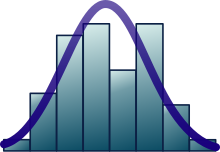
The central limit theorem states that under certain (fairly common) conditions, the sum of many random variables will have an approximately normal distribution.

Cramér's theorem implies that a linear combination of independent non-Gaussian variables will never have an exactly normal distribution, although it may approach it arbitrarily closely.

The standard approach to this problem is the maximum likelihood method, which requires maximization of the log-likelihood function:

This fact is widely used in determining sample sizes for opinion polls and the number of trials in Monte Carlo simulations.

This quantity t has the Student's t-distribution with (n − 1) degrees of freedom, and it is an ancillary statistic (independent of the value of the parameters).

The more prominent of them are outlined below: Diagnostic plots are more intuitively appealing but subjective at the same time, as they rely on informal human judgement to accept or reject the null hypothesis.

In other words, it sums up all possible combinations of products of pairs of elements from x, with a separate coefficient for each.

The above formula reveals why it is more convenient to do Bayesian analysis of conjugate priors for the normal distribution in terms of the precision.

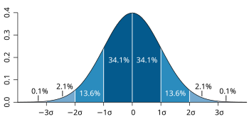
Examples of such quantities are: Approximately normal distributions occur in many situations, as explained by the central limit theorem.

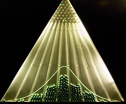
When the outcome is produced by many small effects acting additively and independently, its distribution will be close to normal.

[58] In computer simulations, especially in applications of the Monte-Carlo method, it is often desirable to generate values that are normally distributed.

Some authors[68][69] attribute the discovery of the normal distribution to de Moivre, who in 1738[note 2] published in the second edition of his The Doctrine of Chances the study of the coefficients in the binomial expansion of (a + b)n. De Moivre proved that the middle term in this expansion has the approximate magnitude of

"[70] Although this theorem can be interpreted as the first obscure expression for the normal probability law, Stigler points out that de Moivre himself did not interpret his results as anything more than the approximate rule for the binomial coefficients, and in particular de Moivre lacked the concept of the probability density function.

Not knowing what the function φ is, Gauss requires that his method should reduce to the well-known answer: the arithmetic mean of the measured values.

Using this normal law as a generic model for errors in the experiments, Gauss formulates what is now known as the non-linear weighted least squares method.

[73] Although Gauss was the first to suggest the normal distribution law, Laplace made significant contributions.

[note 4] It was Laplace who first posed the problem of aggregating several observations in 1774,[74] although his own solution led to the Laplacian distribution.

[76] Finally, it was Laplace who in 1810 proved and presented to the academy the fundamental central limit theorem, which emphasized the theoretical importance of the normal distribution.

[77] It is of interest to note that in 1809 an Irish-American mathematician Robert Adrain published two insightful but flawed derivations of the normal probability law, simultaneously and independently from Gauss.

[79] In the middle of the 19th century Maxwell demonstrated that the normal distribution is not just a convenient mathematical tool, but may also occur in natural phenomena:[80] The number of particles whose velocity, resolved in a certain direction, lies between x and x + dx is

Also, it was Pearson who first wrote the distribution in terms of the standard deviation σ as in modern notation.

Soon after this, in year 1915, Fisher added the location parameter to the formula for normal distribution, expressing it in the way it is written nowadays: