Analysis of algorithms

Usually, this involves determining a function that relates the size of an algorithm's input to the number of steps it takes (its time complexity) or the number of storage locations it uses (its space complexity).

An algorithm is said to be efficient when this function's values are small, or grow slowly compared to a growth in the size of the input.

[1] Algorithm analysis is an important part of a broader computational complexity theory, which provides theoretical estimates for the resources needed by any algorithm which solves a given computational problem.

These estimates provide an insight into reasonable directions of search for efficient algorithms.

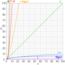
[2] For instance, binary search is said to run in a number of steps proportional to the logarithm of the size n of the sorted list being searched, or in O(log n), colloquially "in logarithmic time".

For example, if the sorted list to which we apply binary search has n elements, and we can guarantee that each lookup of an element in the list can be done in unit time, then at most log2(n) + 1 time units are needed to return an answer.

For the analysis to correspond usefully to the actual run-time, the time required to perform a step must be guaranteed to be bounded above by a constant.

One must be careful here; for instance, some analyses count an addition of two numbers as one step.

For example, if the numbers involved in a computation may be arbitrarily large, the time required by a single addition can no longer be assumed to be constant.

A key point which is often overlooked is that published lower bounds for problems are often given for a model of computation that is more restricted than the set of operations that you could use in practice and therefore there are algorithms that are faster than what would naively be thought possible.

[8] Run-time analysis is a theoretical classification that estimates and anticipates the increase in running time (or run-time or execution time) of an algorithm as its input size (usually denoted as n) increases.

Run-time efficiency is a topic of great interest in computer science: A program can take seconds, hours, or even years to finish executing, depending on which algorithm it implements.

While software profiling techniques can be used to measure an algorithm's run-time in practice, they cannot provide timing data for all infinitely many possible inputs; the latter can only be achieved by the theoretical methods of run-time analysis.

Take as an example a program that looks up a specific entry in a sorted list of size n. Suppose this program were implemented on Computer A, a state-of-the-art machine, using a linear search algorithm, and on Computer B, a much slower machine, using a binary search algorithm.

However, if the size of the input-list is increased to a sufficient number, that conclusion is dramatically demonstrated to be in error: Computer A, running the linear search program, exhibits a linear growth rate.

On the other hand, Computer B, running the binary search program, exhibits a logarithmic growth rate.

Quadrupling the input size only increases the run-time by a constant amount (in this example, 50,000 ns).

Informally, an algorithm can be said to exhibit a growth rate on the order of a mathematical function if beyond a certain input size n, the function f(n) times a positive constant provides an upper bound or limit for the run-time of that algorithm.

In other words, for a given input size n greater than some n0 and a constant c, the run-time of that algorithm will never be larger than c × f(n).

Big O notation is a convenient way to express the worst-case scenario for a given algorithm, although it can also be used to express the average-case — for example, the worst-case scenario for quicksort is O(n2), but the average-case run-time is O(n log n).

Applied to the above table: It is clearly seen that the first algorithm exhibits a linear order of growth indeed following the power rule.

Consider the following pseudocode: A given computer will take a discrete amount of time to execute each of the instructions involved with carrying out this algorithm.

Altogether, the total time required to run the inner loop body can be expressed as an arithmetic progression: which can be factored[11] as The total time required to run the inner loop test can be evaluated similarly: which can be factored as Therefore, the total run-time for this algorithm is: which reduces to As a rule-of-thumb, one can assume that the highest-order term in any given function dominates its rate of growth and thus defines its run-time order.

The methodology of run-time analysis can also be utilized for predicting other growth rates, such as consumption of memory space.

As an example, consider the following pseudocode which manages and reallocates memory usage by a program based on the size of a file which that program manages: In this instance, as the file size n increases, memory will be consumed at an exponential growth rate, which is order O(2n).

This is an extremely rapid and most likely unmanageable growth rate for consumption of memory resources.

In time-sensitive applications, an algorithm taking too long to run can render its results outdated or useless.

An inefficient algorithm can also end up requiring an uneconomical amount of computing power or storage in order to run, again rendering it practically useless.

Analysis of algorithms typically focuses on the asymptotic performance, particularly at the elementary level, but in practical applications constant factors are important, and real-world data is in practice always limited in size.

), but switch to an asymptotically inefficient algorithm (here insertion sort, with time complexity