Born coordinates
This chart is often attributed to Max Born, due to his 1909 work on the relativistic physics of a rotating body.
The world lines of these observers form a timelike congruence which is rigid in the sense of having a vanishing expansion tensor.
is a timelike unit vector field while the others are spacelike unit vector fields; at each event, all four are mutually orthogonal and determine the infinitesimal Lorentz frame of the static observer whose world line passes through that event.
It is defined on the region 0 < R < 1/ω; this limitation is fundamental, since near the outer boundary, the velocity of the Langevin observers approaches the speed of light.
appears in the cylindrical chart as a helix with constant radius (such as the red curve in Fig. 1).
Computing the kinematic decomposition of the Langevin congruence, we find that the acceleration vector is This points radially inward and it depends only on the (constant) radius of each helical world line.
The expansion tensor vanishes identically, which means that nearby Langevin observers maintain constant distance from each other.
Needless to say, in the process of "unwinding" the world lines of the Langevin observers, which appear as helices in the cylindrical chart, we "wound up" the world lines of the static observers, which now appear as helices in the Born chart!
Indeed, it turns out that this is possible, in which case we say the congruence is hypersurface orthogonal, if and only if the vorticity vector vanishes identically.
Thus, while the static observers in the cylindrical chart admits a unique family of orthogonal hyperslices
This is our second (and much more pointed) indication that defining "the spatial geometry of a rotating disk" is not as simple as one might expect.
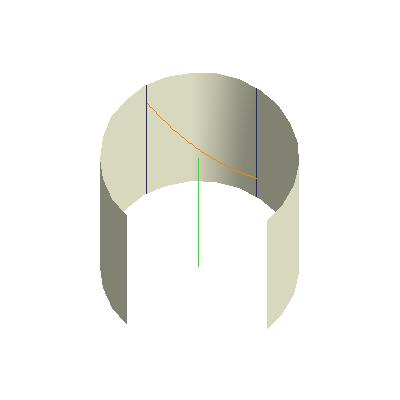
To better understand this crucial point, consider integral curves of the third Langevin frame vector which pass through the radius
That is, it is a kind of infinitesimal obstruction to the existence of a satisfactory notion of spatial hyperslices for our rotating observers.
We wish to compute the round trip travel time, as measured by a ring-riding observer, for a laser pulse sent clockwise and counterclockwise around the cable.
For simplicity, we will ignore the fact that light travels through a fiber optic cable at somewhat less than the speed of light in vacuum, and will pretend that the world line of our laser pulse is a null curve (but certainly not a null geodesic!).
(positive ω means counter-clockwise rotation, negative ω means clockwise rotation) so that the ring-riding observers can determine the angular velocity of the ring (as measured by a static observer) from the difference between clockwise and counterclockwise travel times.
An outward bound radial null geodesic may be written in the form with the radius R0 of the ring riding Langevin observer (see Fig. 4).
Similarly for inward bound radial null geodesics we get depicted as red curve in Fig. 4.
These families of inward and outward bound radial null geodesics represent very different curves in spacetime and their projections do not agree for ω > 0.
Note too that the picture presented here is fully compatible with our expectation (see appearance of the night sky) that a moving observer will see the apparent position of other objects on his celestial sphere to be displaced toward the direction of his motion.
To drive home this crucial point, compare the radar distances obtained by two ring-riding observers with radial coordinate R = R0.
, we now write the coordinates of event A″ as By requiring that the line segments connecting these events be null, we obtain an equation which in principle we can solve for Δ s. It turns out that this procedure gives a rather complicated nonlinear equation, so we simply present some representative numerical results.
Despite these possibly discouraging discrepancies, it is by no means impossible to devise a coordinate chart which is adapted to describing the physical experience of a single Langevin observer, or even a single arbitrarily accelerating observer in Minkowski spacetime.
In the case of steady circular motion, this chart is in fact very closely related to the notion of radar distance "in the large" from a given Langevin observer.
That is, we can consider the quotient space of Minkowski spacetime (or rather, the region 0 < R < 1/ω) by the Langevin congruence, which is a three-dimensional topological manifold.
To see this, consider the Born line element Setting ds2 = 0 and solving for dt we obtain The elapsed proper time for a roundtrip radar blip emitted by a Langevin observer is then Therefore, in our quotient manifold, the Riemannian line element corresponds to distance between infinitesimally nearby Langevin observers.
This metric was first given by Langevin, but the interpretation in terms of radar distance "in the small" is due to Lev Landau and Evgeny Lifshitz, who generalized the construction to work for the quotient of any Lorentzian manifold by a stationary timelike congruence.
If we adopt the coframe we can easily compute the Riemannian curvature tensor of our three-dimensional quotient manifold.
It has only two independent nontrivial components, Thus, in some sense, the geometry of a rotating disk is curved, as Theodor Kaluza claimed (without proof) as early as 1910.
The values given by this notion are in contradiction to the radar distances "in the large" computed in the previous section.