Rindler coordinates
The phenomena in this hyperbolically accelerated frame can be compared to effects arising in a homogeneous gravitational field.
[11] Regarding the history, such coordinates were introduced soon after the advent of special relativity, when they were studied (fully or partially) alongside the concept of hyperbolic motion: In relation to flat Minkowski spacetime by Albert Einstein (1907, 1912),[H 2] Max Born (1909),[H 1] Arnold Sommerfeld (1910),[H 3] Max von Laue (1911),[H 4] Hendrik Lorentz (1913),[H 5] Friedrich Kottler (1914),[H 6] Wolfgang Pauli (1921),[H 7] Karl Bollert (1922),[H 8] Stjepan Mohorovičić (1922),[H 9] Georges Lemaître (1924),[H 10] Einstein & Nathan Rosen (1935),[H 2] Christian Møller (1943, 1952),[H 11] Fritz Rohrlich (1963),[12] Harry Lass (1963),[13] and in relation to both flat and curved spacetime of general relativity by Wolfgang Rindler (1960, 1966).
as constant, so that it represents the simultaneous "rest shape" of a body in hyperbolic motion measured by a comoving observer.
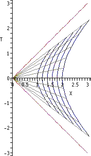
Using the coordinate transformation above, we find that these correspond to hyperbolic arcs in the original Cartesian chart.
The vanishing of the expansion tensor implies that each of our observers maintains constant distance to his neighbors.
The vanishing of the vorticity tensor implies that the world lines of our observers are not twisting about each other; this is a kind of local absence of "swirling".
This may seem surprising because in Newtonian physics, observers who maintain constant relative distance must share the same acceleration.
This leads to a differential equation showing that, at some distance, the acceleration of the trailing end diverges, resulting in the Rindler horizon.
One way to see this is to observe that the magnitude of the acceleration vector is just the path curvature of the corresponding world line.
It is worthwhile to also introduce an alternative frame, given in the Minkowski chart by the natural choice Transforming these vector fields using the coordinate transformation given above, we find that in the Rindler chart (in the Rindler wedge) this frame becomes Computing the kinematic decomposition of the timelike congruence defined by the timelike unit vector field
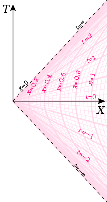
In the Rindler chart, the world lines of the Minkowski observers appear as hyperbolic secant curves asymptotic to the coordinate plane
Specifically, in Rindler coordinates, the world line of the Minkowski observer passing through the event
), we obtain a picture which looks suspiciously like the family of all semicircles through a point and orthogonal to the Rindler horizon (See the figure).
Therefore, we may immediately write down the Fermat metric for the Rindler observers: But this is the well-known line element of hyperbolic three-space H3 in the upper half space chart.
Indeed, in the Cartesian chart we can readily find ten linearly independent Killing vector fields, generating respectively one parameter subgroups of time translation, three spatials, three rotations and three boosts.
We obtain four familiar looking Killing vector fields (time translation, spatial translations orthogonal to the direction of acceleration, and spatial rotation orthogonal to the direction of acceleration) plus six more: (where the signs are chosen consistently + or −).
We will call this the ruler distance since it corresponds to this induced Riemannian metric, but its operational meaning might not be immediately apparent.
The radar distance is then obtained by dividing the round trip travel time, as measured by an ideal clock carried by our observer.
(In Minkowski spacetime, fortunately, we can ignore the possibility of multiple null geodesic paths between two world lines, but in cosmological models and other applications[which?]
in the Rindler line element, we readily obtain the equation of null geodesics moving in the direction of acceleration: Therefore, the radar distance between these two observers is given by This is a bit smaller than the ruler distance, but for nearby observers the discrepancy is negligible.
Because of the simple character of null geodesics in Minkowski spacetime, we can readily determine the optical distance between our pair of Rindler observers (aligned with the direction of acceleration).
There are other notions of distance, but the main point is clear: while the values of these various notions will in general disagree for a given pair of Rindler observers, they all agree that every pair of Rindler observers maintains constant distance.
This is of course incompatible with the relativistic principle that no information having any physical effect can be transmitted faster than the speed of light.
Furthermore, in any thought experiment with time varying forces, whether we "kick" an object or try to accelerate it gradually, we cannot avoid the problem of avoiding mechanical models which are inconsistent with relativistic kinematics (because distant parts of the body respond too quickly to an applied force).
Albert Einstein (1907)[H 13] studied the effects within a uniformly accelerated frame, obtaining equations for coordinate dependent time dilation and speed of light equivalent to (2c), and in order to make the formulas independent of the observer's origin, he obtained time dilation (2i) in formal agreement with Radar coordinates.
Einstein (1912)[H 17] studied a static gravitational field and obtained the Kottler–Møller metric (2b) as well as approximations to formulas (2a) using a coordinate dependent speed of light.
[28] Hendrik Lorentz (1913)[H 18] obtained coordinates similar to (2d, 2e, 2f) while studying Einstein's equivalence principle and the uniform gravitational field.
A detailed description was given by Friedrich Kottler (1914),[H 19] who formulated the corresponding orthonormal tetrad, transformation formulas and metric (2a, 2b).
In a paper concerned with Born rigidity, Georges Lemaître (1924)[H 21] obtained coordinates and metric (2a, 2b).
Albert Einstein and Nathan Rosen (1935) described (2d, 2e) as the "well known" expressions for a homogeneous gravitational field.