Boundary conditions in computational fluid dynamics
Almost every computational fluid dynamics problem is defined under the limits of initial and boundary conditions.
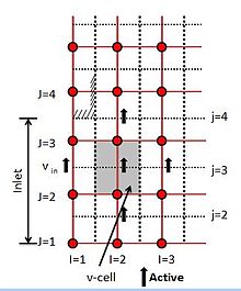
The most common boundary conditions used in computational fluid dynamics are Consider the case of an inlet perpendicular to the x direction.
If flow across the boundary is zero: Normal velocities are set to zero Scalar flux across the boundary is zero: In this type of situations values of properties just adjacent to the solution domain are taken as values at the nearest node just inside the domain.
Consider situation solid wall parallel to the x-direction: Assumptions made and relations considered- Turbulent flow:
Considering the case of an outlet perpendicular to the x-direction - In fully developed flow no changes occurs in flow direction, gradient of all variables except pressure are zero in flow direction The equations are solved for cells up to NI-1, outside the domain values of flow variables are determined by extrapolation from the interior by assuming zero gradients at the outlet plane The outlet plane velocities with the continuity correction