Chaotic scattering
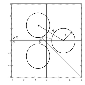
The concept is very simple: we have three hard discs arranged in some triangular formation, a point particle is sent in and undergoes perfect, elastic collisions until it exits towards infinity.
We can calculate the decay rate by simulating the system over many trials and forming a histogram of the delay time, T. For the GR system, it is easy to see that the delay time and the length of the particle trajectory are equivalent but for a multiplication coefficient.
The path-length, s, is equivalent to the decay time, T, provided we scale the (constant) speed appropriately.
Note that an exponential decay rate is a property specifically of hyperbolic chaotic scattering.
As shown by Sweet, Ott and Yorke, [5] a more effective method is to direct coloured light through the gaps between the discs (or in this case, tape coloured strips of paper across pairs of cylinders) and view the reflections through an open gap.
The result is a complex pattern of stripes of alternating colour, as shown below, seen more clearly in the simulated version below that.
Figures 5 and 6 show the basins of attraction for each impact parameter, b, that is, for a given value of b, through which gap does the particle exit?
The basin boundaries form a Cantor set and represent members of the stable manifold: trajectories that, once started, never exit the system.
Note that the totally non-attracting nature of the invariant set is another property of a hyperbolic chaotic scatterer.
Each member of the invariant set can be modelled using symbolic dynamics: the trajectory is labelled based on each of the discs off of which it rebounds.
When you consider that a member of the invariant set must "fit" in the boundaries between two basins of attraction, it is apparent that, if perturbed, the trajectory may exit anywhere along the sequence.
[2][3][8] Because of their unstable nature, it is difficult to access members of the invariant set or the stable manifold directly.
The uncertainty exponent is ideally tailored to measure the fractal dimension of this type of system.
Note that even though the system is two dimensional, a single impact parameter is sufficient to measure the fractal dimension of the stable manifold.
This is demonstrated in Figure 10, which shows the basins of attraction plotted as a function of a dual impact parameter,
From the preceding discussion, it should be apparent that the decay rate, the fractal dimension and the Lyapunov exponents are all related.
The large Lyapunov exponent, for instance, tells us how fast a trajectory in the invariant set will diverge if perturbed.
Similarly, the fractal dimension will give us information about the density of orbits in the invariant set.
Thus we can see that both will affect the decay rate as captured in the following conjecture for a two-dimensional scattering system:[2] where D1 is the information dimension and h1 and h2 are the small and large Lyapunov exponents, respectively.