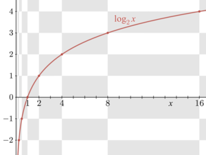
Logarithm
Logarithms are commonplace in scientific formulae, and in measurements of the complexity of algorithms and of geometric objects called fractals.
They help to describe frequency ratios of musical intervals, appear in formulas counting prime numbers or approximating factorials, inform some models in psychophysics, and can aid in forensic accounting.
Similarly, the discrete logarithm is the multi-valued inverse of the exponential function in finite groups; it has uses in public-key cryptography.
(If b is not a positive real number, both exponentiation and logarithm can be defined but may take several values, which makes definitions much more complicated.)
by which tables of logarithms allow multiplication and division to be reduced to addition and subtraction, a great aid to calculations before the invention of computers.
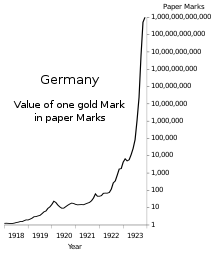
[8] Binary logarithms are also used in computer science, where the binary system is ubiquitous; in music theory, where a pitch ratio of two (the octave) is ubiquitous and the number of cents between any two pitches is a scaled version of the binary logarithm, or log 2 times 1200, of the pitch ratio (that is, 100 cents per semitone in conventional equal temperament), or equivalently the log base 21/1200 ; and in photography rescaled base 2 logarithms are used to measure exposure values, light levels, exposure times, lens apertures, and film speeds in "stops".
[13] The history of logarithms in seventeenth-century Europe saw the discovery of a new function that extended the realm of analysis beyond the scope of algebraic methods.
[19][20] Prior to Napier's invention, there had been other techniques of similar scopes, such as the prosthaphaeresis or the use of tables of progressions, extensively developed by Jost Bürgi around 1600.
[21][22] Napier coined the term for logarithm in Middle Latin, logarithmus, literally meaning 'ratio-number', derived from the Greek logos 'proportion, ratio, word' + arithmos 'number'.
[24] The first real logarithms were heuristic methods to turn multiplication into addition, thus facilitating rapid computation.
Invention of the function now known as the natural logarithm began as an attempt to perform a quadrature of a rectangular hyperbola by Grégoire de Saint-Vincent, a Belgian Jesuit residing in Prague.
Before Euler developed his modern conception of complex natural logarithms, Roger Cotes had a nearly equivalent result when he showed in 1714 that[27]
Tables of logarithms need only include the mantissa, as the characteristic can be easily determined by counting digits from the decimal point.
William Oughtred enhanced it to create the slide rule—a pair of logarithmic scales movable with respect to each other.
The slide rule was an essential calculating tool for engineers and scientists until the 1970s, because it allows, at the expense of precision, much faster computation than techniques based on tables.
It is a standard result in real analysis that any continuous strictly monotonic function is bijective between its domain and range.
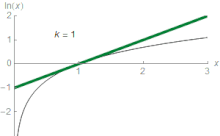
That is, the slope of the tangent touching the graph of the base-b logarithm at the point (x, logb (x)) equals 1/(x ln(b)).
[48][49] Moreover, the binary logarithm algorithm calculates lb(x) recursively, based on repeated squarings of x, taking advantage of the relation
The nth partial sum can approximate ln(z) with arbitrary precision, provided the number of summands n is large enough.
While at Los Alamos National Laboratory working on the Manhattan Project, Richard Feynman developed a bit-processing algorithm to compute the logarithm that is similar to long division and was later used in the Connection Machine.
It is used to quantify the attenuation or amplification of electrical signals,[57] to describe power levels of sounds in acoustics,[58] and the absorbance of light in the fields of spectrometry and optics.
The signal-to-noise ratio describing the amount of unwanted noise in relation to a (meaningful) signal is also measured in decibels.
[59] In a similar vein, the peak signal-to-noise ratio is commonly used to assess the quality of sound and image compression methods using the logarithm.
In such graphs, exponential functions of the form f(x) = a · bx appear as straight lines with slope equal to the logarithm of b. Log-log graphs scale both axes logarithmically, which causes functions of the form f(x) = a · xk to be depicted as straight lines with slope equal to the exponent k. This is applied in visualizing and analyzing power laws.
[69] In psychophysics, the Weber–Fechner law proposes a logarithmic relationship between stimulus and sensation such as the actual vs. the perceived weight of an item a person is carrying.
According to Benford's law, the probability that the first decimal-digit of an item in the data sample is d (from 1 to 9) equals log10 (d + 1) − log10 (d), regardless of the unit of measurement.
In other words, the amount of memory needed to store N grows logarithmically with N. Entropy is broadly a measure of the disorder of some system.
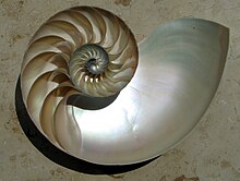
[88] Fractals are geometric objects that are self-similar in the sense that small parts reproduce, at least roughly, the entire global structure.
Another logarithm-based notion of dimension is obtained by counting the number of boxes needed to cover the fractal in question.
The Riemann hypothesis, one of the oldest open mathematical conjectures, can be stated in terms of comparing π(x) and Li(x).