Vector space

Around 1636, French mathematicians René Descartes and Pierre de Fermat founded analytic geometry by identifying solutions to an equation of two variables with points on a plane curve.

[18] To achieve geometric solutions without using coordinates, Bolzano introduced, in 1804, certain operations on points, lines, and planes, which are predecessors of vectors.

[22] Vectors were reconsidered with the presentation of complex numbers by Argand and Hamilton and the inception of quaternions by the latter.

In 1857, Cayley introduced the matrix notation which allows for harmonization and simplification of linear maps.

Grassmann's 1844 work exceeds the framework of vector spaces as well since his considering multiplication led him to what are today called algebras.

In 1897, Salvatore Pincherle adopted Peano's axioms and made initial inroads into the theory of infinite-dimensional vector spaces.

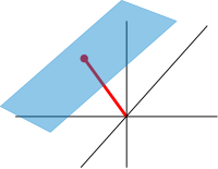
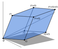
[31] The following shows a few examples: if a = 2, the resulting vector aw has the same direction as w, but is stretched to the double length of w (the second image).

Equivalently, 2w is the sum w + w. Moreover, (−1)v = −v has the opposite direction and the same length as v (blue vector pointing down in the second image).

Functions from any fixed set Ω to a field F also form vector spaces, by performing addition and scalar multiplication pointwise.

Such function spaces occur in many geometric situations, when Ω is the real line or an interval, or other subsets of R. Many notions in topology and analysis, such as continuity, integrability or differentiability are well-behaved with respect to linearity: sums and scalar multiples of functions possessing such a property still have that property.

They form a vector space: sums and scalar multiples of such triples still satisfy the same ratios of the three variables; thus they are solutions, too.

In a similar vein, the solutions of homogeneous linear differential equations form vector spaces.

They are functions that reflect the vector space structure, that is, they preserve sums and scalar multiplication:

[38] If there exists an isomorphism between V and W, the two spaces are said to be isomorphic; they are then essentially identical as vector spaces, since all identities holding in V are, via f, transported to similar ones in W, and vice versa via g. For example, the arrows in the plane and the ordered pairs of numbers vector spaces in the introduction above (see § Examples) are isomorphic: a planar arrow v departing at the origin of some (fixed) coordinate system can be expressed as an ordered pair by considering the x- and y-component of the arrow, as shown in the image at the right.

Another way to express this is that any vector space over a given field is completely classified (up to isomorphism) by its dimension, a single number.

[47] The linear transformation of Rn corresponding to a real n-by-n matrix is orientation preserving if and only if its determinant is positive.

In addition to the above concrete examples, there are a number of standard linear algebraic constructions that yield vector spaces related to given ones.

[57] The existence of kernels and images is part of the statement that the category of vector spaces (over a fixed field

and the second and third isomorphism theorem can be formulated and proven in a way very similar to the corresponding statements for groups.

It is defined as the vector space consisting of finite (formal) sums of symbols called tensors

Likewise, linear algebra is not adapted to deal with infinite series, since the addition operation allows only finitely many terms to be added.

The fundamental Hahn–Banach theorem is concerned with separating subspaces of appropriate topological vector spaces by continuous functionals.

[80] A similar approximation technique by trigonometric functions is commonly called Fourier expansion, and is much applied in engineering.

[83] Definite values for physical properties such as energy, or momentum, correspond to eigenvalues of a certain (linear) differential operator and the associated wavefunctions are called eigenstates.

The spectral theorem decomposes a linear compact operator acting on functions in terms of these eigenfunctions and their eigenvalues.

[86] Another crucial example are Lie algebras, which are neither commutative nor associative, but the failure to be so is limited by the constraints (

[nb 12] In contrast, by the hairy ball theorem, there is no (tangent) vector field on the 2-sphere S2 which is everywhere nonzero.

[94] The theory of modules, compared to that of vector spaces, is complicated by the presence of ring elements that do not have multiplicative inverses.

[95] The algebro-geometric interpretation of commutative rings via their spectrum allows the development of concepts such as locally free modules, the algebraic counterpart to vector bundles.

generalizing the homogeneous case discussed in the above section on linear equations, which can be found by setting