Compressed sensing
[1][2] Compressed sensing has applications in, for example, magnetic resonance imaging (MRI) where the incoherence condition is typically satisfied.
-norm was also used in signal processing, for example, in the 1970s, when seismologists constructed images of reflective layers within the earth based on data that did not seem to satisfy the Nyquist–Shannon criterion.
In compressed sensing, one adds the constraint of sparsity, allowing only solutions which have a small number of nonzero coefficients.
The results found by Emmanuel Candès, Justin Romberg, Terence Tao, and David Donoho showed that the number of these compressive measurements can be small and still contain nearly all the useful information.
However, adding the constraint that the initial signal is sparse enables one to solve this underdetermined system of linear equations.
To enforce the sparsity constraint when solving for the underdetermined system of linear equations, one can minimize the number of nonzero components of the solution.
The current CS Regularization models attempt to address this problem by incorporating sparsity priors of the original image, one of which is the total variation (TV).
[14] TV methods with iterative re-weighting have been implemented to reduce the influence of large gradient value magnitudes in the images.
However, as gradient magnitudes are used for estimation of relative penalty weights between the data fidelity and regularization terms, this method is not robust to noise and artifacts and accurate enough for CS image/signal reconstruction and, therefore, fails to preserve smaller structures.
One of the disadvantages is the need for defining a valid starting point as a global minimum might not be obtained every time due to the concavity of the function.
The advantages of this method include: reduction of the sampling rate for sparse signals; reconstruction of the image while being robust to the removal of noise and other artifacts; and use of very few iterations.
In the figure shown below, P1 refers to the first-step of the iterative reconstruction process, of the projection matrix P of the fan-beam geometry, which is constrained by the data fidelity term.
Furthermore, using these insufficient projections in standard TV algorithms end up making the problem under-determined and thus leading to infinitely many possible solutions.
This allows for easier detection of sharp discontinuities in intensity in the images and thereby adapt the weight to store the recovered edge information during the process of signal/image reconstruction.
To prevent over-smoothing of edges and texture details and to obtain a reconstructed CS image which is accurate and robust to noise and artifacts, this method is used.
This orientation field is introduced into the directional total variation optimization model for CS reconstruction through the equation:
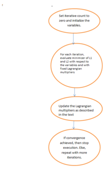
These equations are reduced to a series of convex minimization problems which are then solved with a combination of variable splitting and augmented Lagrangian (FFT-based fast solver with a closed form solution) methods.
For the iterative directional total variation refinement model, the augmented lagrangian method involves initializing
And as in the field refinement model, the lagrangian multipliers are updated and the iterative process is stopped when convergence is achieved.
Based on peak signal-to-noise ratio (PSNR) and structural similarity index (SSIM) metrics and known ground-truth images for testing performance, it is concluded that iterative directional total variation has a better reconstructed performance than the non-iterative methods in preserving edge and texture areas.
Its broad scope and generality has enabled several innovative CS-enhanced approaches in signal processing and compression, solution of inverse problems, design of radiating systems, radar and through-the-wall imaging, and antenna characterization.
[22] Imaging techniques having a strong affinity with compressive sensing include coded aperture and computational photography.
[26] Bell Labs employed the technique in a lensless single-pixel camera that takes stills using repeated snapshots of randomly chosen apertures from a grid.
[27][28] Compressed sensing can be used to improve image reconstruction in holography by increasing the number of voxels one can infer from a single hologram.
[35] Compressed sensing has been used[36][37] to shorten magnetic resonance imaging scanning sessions on conventional hardware.
[38] Reconstruction methods include Compressed sensing addresses the issue of high scan time by enabling faster acquisition by measuring fewer Fourier coefficients.
Compressed sensing, in this case, removes the high spatial gradient parts – mainly, image noise and artifacts.
This holds potential as one can obtain high-resolution CT images at low radiation doses (through lower current-mA settings).
In radio astronomy and optical astronomical interferometry, full coverage of the Fourier plane is usually absent and phase information is not obtained in most hardware configurations.
Compressed sensing combined with a moving aperture has been used to increase the acquisition rate of images in a transmission electron microscope.