Determinant

is denoted either by "det" or by vertical bars around the matrix, and is defined as For example, The determinant has several key properties that can be proved by direct evaluation of the definition for

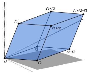
To show that ad − bc is the signed area, one may consider a matrix containing two vectors u ≡ (a, c) and v ≡ (b, d) representing the parallelogram's sides.

Due to the sine this already is the signed area, yet it may be expressed more conveniently using the cosine of the complementary angle to a perpendicular vector, e.g. u⊥ = (−c, a), so that |u⊥| |v| cos θ′ becomes the signed area in question, which can be determined by the pattern of the scalar product to be equal to ad − bc according to the following equations: Thus the determinant gives the scaling factor and the orientation induced by the mapping represented by A.

The signs are determined by how many transpositions of factors are necessary to arrange the factors in increasing order of their columns (given that the terms are arranged left-to-right in increasing row order): positive for an even number of transpositions and negative for an odd number.

The rule of Sarrus is a mnemonic for the expanded form of this determinant: the sum of the products of three diagonal north-west to south-east lines of matrix elements, minus the sum of the products of three diagonal south-west to north-east lines of elements, when the copies of the first two columns of the matrix are written beside it as in the illustration.

While less technical in appearance, this characterization cannot entirely replace the Leibniz formula in defining the determinant, since without it the existence of an appropriate function is not clear.

In fact, Gaussian elimination can be applied to bring any matrix into upper triangular form, and the steps in this algorithm affect the determinant in a controlled way.

-th column is the equality Laplace expansion can be used iteratively for computing determinants, but this approach is inefficient for large matrices.

Brunn–Minkowski theorem implies that the nth root of determinant is a concave function, when restricted to Hermitian positive-definite

That is, for generic n, detA = (−1)nc0 the signed constant term of the characteristic polynomial, determined recursively from In the general case, this may also be obtained from[20] where the sum is taken over the set of all integers kl ≥ 0 satisfying the equation The formula can be expressed in terms of the complete exponential Bell polynomial of n arguments sl = −(l – 1)!

tr(Al) as This formula can also be used to find the determinant of a matrix AIJ with multidimensional indices I = (i1, i2, ..., ir) and J = (j1, j2, ..., jr).

More generally, if is expanded as a formal power series in s then all coefficients of sm for m > n are zero and the remaining polynomial is det(I + sA).

For a positive definite matrix A, the trace operator gives the following tight lower and upper bounds on the log determinant with equality if and only if A = I.

The Leibniz formula shows that the determinant of real (or analogously for complex) square matrices is a polynomial function from

[22] Determinants proper originated separately from the work of Seki Takakazu in 1683 in Japan and parallelly of Leibniz in 1693.

[27] Both Cramer and also Bézout (1779) were led to determinants by the question of plane curves passing through a given set of points.

[24] Laplace (1772) gave the general method of expanding a determinant in terms of its complementary minors: Vandermonde had already given a special case.

[29] Immediately following, Lagrange (1773) treated determinants of the second and third order and applied it to questions of elimination theory; he proved many special cases of general identities.

He introduced the word "determinant" (Laplace had used "resultant"), though not in the present signification, but rather as applied to the discriminant of a quantic.

In this he used the word "determinant" in its present sense,[31][32] summarized and simplified what was then known on the subject, improved the notation, and gave the multiplication theorem with a proof more satisfactory than Binet's.

time, which is comparable to more common methods of solving systems of linear equations, such as LU, QR, or singular value decomposition.

For instance, an orthogonal matrix with entries in Rn represents an orthonormal basis in Euclidean space, and hence has determinant of ±1 (since all the vectors have length 1).

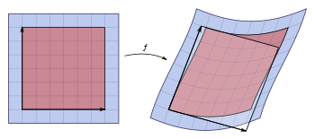
More generally, if the determinant of A is positive, A represents an orientation-preserving linear transformation (if A is an orthogonal 2 × 2 or 3 × 3 matrix, this is a rotation), while if it is negative, A switches the orientation of the basis.

of a field extension, as well as the Pfaffian of a skew-symmetric matrix and the reduced norm of a central simple algebra, also arise as special cases of this construction.

Functional analysis provides different extensions of the determinant for such infinite-dimensional situations, which however only work for particular kinds of operators.

For matrices over non-commutative rings, multilinearity and alternating properties are incompatible for n ≥ 2,[48] so there is no good definition of the determinant in this setting.

For some classes of matrices with non-commutative elements, one can define the determinant and prove linear algebra theorems that are very similar to their commutative analogs.

They are rarely calculated explicitly in numerical linear algebra, where for applications such as checking invertibility and finding eigenvalues the determinant has largely been supplanted by other techniques.

[51] While the determinant can be computed directly using the Leibniz rule this approach is extremely inefficient for large matrices, since that formula requires calculating

is based on the following idea: one replaces permutations (as in the Leibniz rule) by so-called closed ordered walks, in which several items can be repeated.