Hierarchical clustering
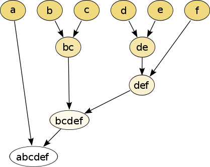
The results of hierarchical clustering[1] are usually presented in a dendrogram.
Hierarchical clustering has the distinct advantage that any valid measure of distance can be used.
On the other hand, except for the special case of single-linkage distance, none of the algorithms (except exhaustive search in
[citation needed] The standard algorithm for hierarchical agglomerative clustering (HAC) has a time complexity of
memory, which makes it too slow for even medium data sets.
However, for some special cases, optimal efficient agglomerative methods (of complexity
) are known: SLINK[2] for single-linkage and CLINK[3] for complete-linkage clustering.
In many cases, the memory overheads of this approach are too large to make it practically usable.
, but it is common to use faster heuristics to choose splits, such as k-means.
In order to decide which clusters should be combined (for agglomerative), or where a cluster should be split (for divisive), a measure of dissimilarity between sets of observations is required.
In most methods of hierarchical clustering, this is achieved by use of an appropriate distance d, such as the Euclidean distance, between single observations of the data set, and a linkage criterion, which specifies the dissimilarity of sets as a function of the pairwise distances of observations in the sets.
The choice of metric as well as linkage can have a major impact on the result of the clustering, where the lower level metric determines which objects are most similar, whereas the linkage criterion influences the shape of the clusters.
For example, complete-linkage tends to produce more spherical clusters than single-linkage.
Some commonly used linkage criteria between two sets of observations A and B and a distance d are:[5][6] Some of these can only be recomputed recursively (WPGMA, WPGMC), for many a recursive computation with Lance-Williams-equations is more efficient, while for other (Hausdorff, Medoid) the distances have to be computed with the slower full formula.
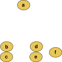
In this example, cutting after the second row (from the top) of the dendrogram will yield clusters {a} {b c} {d e} {f}.
This method builds the hierarchy from the individual elements by progressively merging clusters.
The first step is to determine which elements to merge in a cluster.
Optionally, one can also construct a distance matrix at this stage, where the number in the i-th row j-th column is the distance between the i-th and j-th elements.
is one of the following: In case of tied minimum distances, a pair is randomly chosen, thus being able to generate several structurally different dendrograms.
Alternatively, all tied pairs may be joined at the same time, generating a unique dendrogram.
However, this is not the case of, e.g., the centroid linkage where the so-called reversals[19] (inversions, departures from ultrametricity) may occur.
DIANA chooses the object with the maximum average dissimilarity and then moves all objects to this cluster that are more similar to the new cluster than to the remainder.
Such objects will likely start their own splinter group eventually.
The dendrogram of DIANA can be constructed by letting the splinter group