Ekman layer
Ekman layers occur both in the atmosphere and in the ocean.
The second type occurs at the bottom of the atmosphere and ocean, where frictional forces are associated with flow over rough surfaces.
Ekman developed the theory of the Ekman layer after Fridtjof Nansen observed that ice drifts at an angle of 20°–40° to the right of the prevailing wind direction while on an Arctic expedition aboard the Fram.
Nansen asked his colleague, Vilhelm Bjerknes to set one of his students upon study of the problem.
Bjerknes tapped Ekman, who presented his results in 1902 as his doctoral thesis.
[1] The mathematical formulation of the Ekman layer begins by assuming a neutrally stratified fluid, a balance between the forces of pressure gradient, Coriolis and turbulent drag.
is the diffusive eddy viscosity, which can be derived using mixing length theory.
There are many regions where an Ekman layer is theoretically plausible; they include the bottom of the atmosphere, near the surface of the earth and ocean, the bottom of the ocean, near the sea floor and at the top of the ocean, near the air-water interface.
Each of these situations can be accounted for through the boundary conditions applied to the resulting system of ordinary differential equations.
The separate cases of top and bottom boundary layers are shown below.
We will consider boundary conditions of the Ekman layer in the upper ocean:[2] where
, of the wind field or ice layer at the top of the ocean, and
is called the Ekman layer depth, and gives an indication of the penetration depth of wind-induced turbulent mixing in the ocean.
Note that it varies on two parameters: the turbulent diffusivity
This Ekman depth prediction does not always agree precisely with observations.
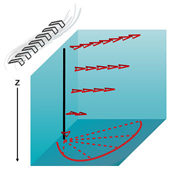
By applying the continuity equation we can have the vertical velocity as following Note that when vertically-integrated, the volume transport associated with the Ekman spiral is to the right of the wind direction in the Northern Hemisphere.
The traditional development of Ekman layers bounded below by a surface utilizes two boundary conditions: There is much difficulty associated with observing the Ekman layer for two main reasons: the theory is too simplistic as it assumes a constant eddy viscosity, which Ekman himself anticipated,[3] saying It is obvious that
cannot generally be regarded as a constant when the density of water is not uniform within the region consideredand because it is difficult to design instruments with great enough sensitivity to observe the velocity profile in the ocean.
The bottom Ekman layer can readily be observed in a rotating cylindrical tank of water by dropping in dye and changing the rotation rate slightly.
[4] Surface Ekman layers can also be observed in rotating tanks.
[5] In the atmosphere, the Ekman solution generally overstates the magnitude of the horizontal wind field because it does not account for the velocity shear in the surface layer.
The Ekman layer near the surface of the ocean extends only about 10 – 20 meters deep,[6] and instrumentation sensitive enough to observe a velocity profile in such a shallow depth has only been available since around 1980.
[7] Observations of the Ekman layer have only been possible since the development of robust surface moorings and sensitive current meters.
Ekman himself developed a current meter to observe the spiral that bears his name, but was not successful.
[10] More recent observations include (not an exhaustive list): Common to several of these observations spirals were found to be "compressed", displaying larger estimates of eddy viscosity when considering the rate of rotation with depth than the eddy viscosity derived from considering the rate of decay of speed.