Hidden Markov model
Hidden Markov models are known for their applications to thermodynamics, statistical mechanics, physics, chemistry, economics, finance, signal processing, information theory, pattern recognition—such as speech,[1] handwriting, gesture recognition,[2] part-of-speech tagging, musical score following,[3] partial discharges[4] and bioinformatics.
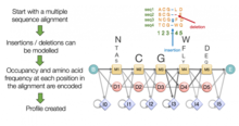
This is illustrated by the lower part of the diagram shown in Figure 1, where one can see that balls y1, y2, y3, y4 can be drawn at each state.
Consider two friends, Alice and Bob, who live far apart from each other and who talk together daily over the telephone about what they did that day.
On each day, there is a certain chance that Bob will perform one of the following activities, depending on the weather: "walk", "shop", or "clean".
In the standard type of hidden Markov model considered here, the state space of the hidden variables is discrete, while the observations themselves can either be discrete (typically generated from a categorical distribution) or continuous (typically from a Gaussian distribution).
The hidden state space is assumed to consist of one of N possible values, modelled as a categorical distribution.
For example, if the observed variable is discrete with M possible values, governed by a categorical distribution, there will be
A number of related tasks ask about the probability of one or more of the latent variables, given the model's parameters and a sequence of observations
This is similar to filtering but asks about the distribution of a latent variable somewhere in the middle of a sequence, i.e. to compute
From the perspective described above, this can be thought of as the probability distribution over hidden states for a point in time k in the past, relative to time t. The forward-backward algorithm is a good method for computing the smoothed values for all hidden state variables.
An example is part-of-speech tagging, where the hidden states represent the underlying parts of speech corresponding to an observed sequence of words.
This task requires finding a maximum over all possible state sequences, and can be solved efficiently by the Viterbi algorithm.
The task is usually to derive the maximum likelihood estimate of the parameters of the HMM given the set of output sequences.
If the HMMs are used for time series prediction, more sophisticated Bayesian inference methods, like Markov chain Monte Carlo (MCMC) sampling are proven to be favorable over finding a single maximum likelihood model both in terms of accuracy and stability.
[9] Since MCMC imposes significant computational burden, in cases where computational scalability is also of interest, one may alternatively resort to variational approximations to Bayesian inference, e.g.[10] Indeed, approximate variational inference offers computational efficiency comparable to expectation-maximization, while yielding an accuracy profile only slightly inferior to exact MCMC-type Bayesian inference.
Applications include: Hidden Markov models were described in a series of statistical papers by Leonard E. Baum and other authors in the second half of the 1960s.
[34][35][36][37] From the linguistics point of view, hidden Markov models are equivalent to stochastic regular grammar.
[40] In the hidden Markov models considered above, the state space of the hidden variables is discrete, while the observations themselves can either be discrete (typically generated from a categorical distribution) or continuous (typically from a Gaussian distribution).
Typically, a symmetric Dirichlet distribution is chosen, reflecting ignorance about which states are inherently more likely than others.
Values greater than 1 produce a dense matrix, in which the transition probabilities between pairs of states are likely to be nearly equal.
The parameters of models of this sort, with non-uniform prior distributions, can be learned using Gibbs sampling or extended versions of the expectation-maximization algorithm.
It was originally described under the name "Infinite Hidden Markov Model"[43] and was further formalized in "Hierarchical Dirichlet Processes".
Finally, arbitrary features over pairs of adjacent hidden states can be used rather than simple transition probabilities.
The disadvantages of such models are: (1) The types of prior distributions that can be placed on hidden states are severely limited; (2) It is not possible to predict the probability of seeing an arbitrary observation.
This second limitation is often not an issue in practice, since many common usages of HMM's do not require such predictive probabilities.
The advantage of this type of model is that it does not suffer from the so-called label bias problem of MEMM's, and thus may make more accurate predictions.
This information, encoded in the form of a high-dimensional vector, is used as a conditioning variable of the HMM state transition probabilities.
Under such a setup, eventually is obtained a nonstationary HMM, the transition probabilities of which evolve over time in a manner that is inferred from the data, in contrast to some unrealistic ad-hoc model of temporal evolution.
[54][55] Unlike traditional methods such as the Forward-Backward and Viterbi algorithms, which require knowledge of the joint law of the HMM and can be computationally intensive to learn, the Discriminative Forward-Backward and Discriminative Viterbi algorithms circumvent the need for the observation's law.
A complete overview of the latent Markov models, with special attention to the model assumptions and to their practical use is provided in[59] Given a Markov transition matrix and an invariant distribution on the states, a probability measure can be imposed on the set of subshifts.
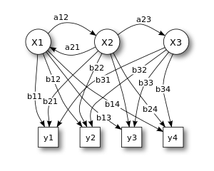
X — states
y — possible observations
a — state transition probabilities
b — output probabilities


5 3 2 5 3 2
4 3 2 5 3 2
3 1 2 5 3 2
The most likely sequence can be found by evaluating the joint probability of both the state sequence and the observations for each case (simply by multiplying the probability values, which here correspond to the opacities of the arrows involved). In general, this type of problem (i.e., finding the most likely explanation for an observation sequence) can be solved efficiently using the Viterbi algorithm .