Singular value decomposition
To get a more visual flavor of singular values and SVD factorization – at least when working on real vector spaces – consider the sphere
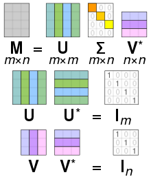
are unitary, multiplying by their respective conjugate transposes yields identity matrices, as shown below.
are multiplied by zero, so have no effect on the matrix product, and can be replaced by any unit vectors which are orthogonal to the first three and to each-other.
Non-degenerate singular values always have unique left- and right-singular vectors, up to multiplication by a unit-phase factor
In general, the SVD is unique up to arbitrary unitary transformations applied uniformly to the column vectors of both
being a normal matrix, and thus also square, the spectral theorem ensures that it can be unitarily diagonalized using a basis of eigenvectors, and thus decomposed as
It also means that if there are several vanishing singular values, any linear combination of the corresponding right-singular vectors is a valid solution.
The SVD can be thought of as decomposing a matrix into a weighted, ordered sum of separable matrices.
[6][7][8][9] The SVD is also applied extensively to the study of linear inverse problems and is useful in the analysis of regularization methods such as that of Tikhonov.
[10][11] The SVD also plays a crucial role in the field of quantum information, in a form often referred to as the Schmidt decomposition.
Through it, states of two quantum systems are naturally decomposed, providing a necessary and sufficient condition for them to be entangled: if the rank of the
One application of SVD to rather large matrices is in numerical weather prediction, where Lanczos methods are used to estimate the most linearly quickly growing few perturbations to the central numerical weather prediction over a given initial forward time period; i.e., the singular vectors corresponding to the largest singular values of the linearized propagator for the global weather over that time interval.
These perturbations are then run through the full nonlinear model to generate an ensemble forecast, giving a handle on some of the uncertainty that should be allowed for around the current central prediction.
SVD was coupled with radial basis functions to interpolate solutions to three-dimensional unsteady flow problems.
[12] Interestingly, SVD has been used to improve gravitational waveform modeling by the ground-based gravitational-wave interferometer aLIGO.
[17] In astrodynamics, the SVD and its variants are used as an option to determine suitable maneuver directions for transfer trajectory design[18] and orbital station-keeping.
Similar to the eigenvalues case, by assumption the two vectors satisfy the Lagrange multiplier equation:
The iterations proceeds exactly as in the Jacobi eigenvalue algorithm: by cyclic sweeps over all off-diagonal elements.
The second step can be done by a variant of the QR algorithm for the computation of eigenvalues, which was first described by Golub & Kahan (1965).
The LAPACK subroutine DBDSQR[22] implements this iterative method, with some modifications to cover the case where the singular values are very small (Demmel & Kahan 1990).
Yet another method for step 2 uses the idea of divide-and-conquer eigenvalue algorithms (Trefethen & Bau III 1997, Lecture 31).
The approaches that use eigenvalue decompositions are based on the QR algorithm, which is well-developed to be stable and fast.
of the non-zero singular values is large making even the Compact SVD impractical to compute.
This is an important property for applications in which it is necessary to preserve Euclidean distances and invariance with respect to rotations.
As for matrices, the singular value factorization is equivalent to the polar decomposition for operators: we can simply write
The notion of singular values and left/right-singular vectors can be extended to compact operator on Hilbert space as they have a discrete spectrum.
An immediate consequence of this is: The singular value decomposition was originally developed by differential geometers, who wished to determine whether a real bilinear form could be made equal to another by independent orthogonal transformations of the two spaces it acts on.
James Joseph Sylvester also arrived at the singular value decomposition for real square matrices in 1889, apparently independently of both Beltrami and Jordan.
The first proof of the singular value decomposition for rectangular and complex matrices seems to be by Carl Eckart and Gale J.
However, these were replaced by the method of Gene Golub and William Kahan published in 1965,[31] which uses Householder transformations or reflections.

- Top: The action of M , indicated by its effect on the unit disc D and the two canonical unit vectors e 1 and e 2 .
- Left: The action of V ⁎ , a rotation, on D , e 1 , and e 2 .
- Bottom: The action of Σ , a scaling by the singular values σ 1 horizontally and σ 2 vertically.
- Right: The action of U , another rotation.