Linking number
In Euclidean space, the linking number is always an integer, but may be positive or negative depending on the orientation of the two curves (this is not true for curves in most 3-manifolds, where linking numbers can also be fractions or just not exist at all).
It is an important object of study in knot theory, algebraic topology, and differential geometry, and has numerous applications in mathematics and science, including quantum mechanics, electromagnetism, and the study of DNA supercoiling.
Any two closed curves in space, if allowed to pass through themselves but not each other, can be moved into exactly one of the following standard positions.
This is formalized as regular homotopy, which further requires that each curve be an immersion, not just any map.
However, this added condition does not change the definition of linking number (it does not matter if the curves are required to always be immersions or not), which is an example of an h-principle (homotopy-principle), meaning that geometry reduces to topology.
This fact (that the linking number is the only invariant) is most easily proven by placing one circle in standard position, and then showing that linking number is the only invariant of the other circle.
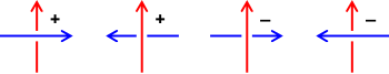
involves only the undercrossings of the blue curve by the red, while
from the torus to the sphere by Pick a point in the unit sphere, v, so that orthogonal projection of the link to the plane perpendicular to v gives a link diagram.
Observe that a point (s, t) that goes to v under the Gauss map corresponds to a crossing in the link diagram where
Thus in order to compute the linking number of the diagram corresponding to v it suffices to count the signed number of times the Gauss map covers v. Since v is a regular value, this is precisely the degree of the Gauss map (i.e. the signed number of times that the image of Γ covers the sphere).
This formulation of the linking number of γ1 and γ2 enables an explicit formula as a double line integral, the Gauss linking integral: This integral computes the total signed area of the image of the Gauss map (the integrand being the Jacobian of Γ) and then divides by the area of the sphere (which is 4π).
In quantum field theory, Gauss's integral definition arises when computing the expectation value of the Wilson loop observable in
Explicitly, the abelian Chern–Simons action for a gauge potential one-form
Since the theory is just Gaussian, no ultraviolet regularization or renormalization is needed.
The only thing left to do is provide an overall normalization factor, and a natural choice will present itself.
The classical equations of motion are Here, we have coupled the Chern–Simons field to a source with a term
Since we are in 3 dimensions, we can rewrite the equations of motion in a more familiar notation: Taking the curl of both sides and choosing Lorenz gauge
, the equations become From electrostatics, the solution is The path integral for arbitrary
, it is clear that there will be terms describing the self-interaction of the particles, and these are uninteresting since they would be there even in the presence of just one loop.
Therefore, we normalize the path integral by a factor precisely cancelling these terms.
Going through the algebra, we obtain where which is simply Gauss's linking integral.
This also served as a hint that the nonabelian variant of Chern–Simons theory computes other knot invariants, and it was shown explicitly by Edward Witten that the nonabelian theory gives the invariant known as the Jones polynomial.
[3] The Chern-Simons gauge theory lives in 3 spacetime dimensions.
More generally, there exists higher dimensional topological quantum field theories.
There exists more complicated multi-loop/string-braiding statistics of 4-dimensional gauge theories captured by the link invariants of exotic topological quantum field theories in 4 spacetime dimensions.