Logistic map
[2] Other researchers who have contributed to the study of the logistic map include Stanisław Ulam, John von Neumann, Pekka Myrberg, Oleksandr Sharkovsky, Nicholas Metropolis, and Mitchell Feigenbaum.
Many chaotic systems such as the Mandelbrot set are emerging from iteration of very simple quadratic non linear functions such as the logistic map.
[May, Robert M. (1976) 2] This nonlinear difference equation is intended to capture two effects: The usual values of interest for the parameter r are those in the interval [0, 4], so that xn remains bounded on [0, 1].
In this case, the variable x of the logistic map is the number of individuals of an organism divided by the maximum population size, so the possible values of x are limited to 0 ≤ x ≤ 1.
, the orbit no longer converges to a single point, but instead alternates between large and small values even after a sufficient amount of time has passed.
Roughly speaking, chaos is a complex and irregular behavior that occurs despite the fact that the difference equation describing the logistic map has no probabilistic ambiguity and the next state is completely and uniquely determined.
For a logistic map with a specific parameter a, an exact solution that explicitly includes the time n and the initial value x 0 has been obtained as follows.
When r = 4 When r = 2 When r = −2 Considering the three exact solutions above, all of them are The relative simplicity of the logistic map makes it a widely used point of entry into a consideration of the concept of chaos.
A rough description of chaos is that chaotic systems exhibits:[Devaney 1989 3][19] These are properties of the logistic map for most values of r between about 3.57 and 4 (as noted above).
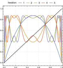
[May, Robert M. (1976) 1] A common source of such sensitivity to initial conditions is that the map represents a repeated folding and stretching of the space on which it is defined.
Figure (b), right, demonstrates this, showing how initially nearby points begin to diverge, particularly in those regions of xt corresponding to the steeper sections of the plot.
This quality of unpredictability and apparent randomness led the logistic map equation to be used as a pseudo-random number generator in early computers.
In general, if a one-dimensional map with one parameter and one variable is unimodal and the vertex can be approximated by a second-order polynomial, then, regardless of the specific form of the map, an infinite period-doubling cascade of bifurcations will occur for the parameter range 3 ≤ r ≤ 3.56994... , and the ratio δ defined by equation ( 3-13 ) is equal to the Feigenbaum constant, 4.669... .
By universality, we can use another family of functions that also undergoes repeated period-doubling on its route to chaos, and even though it is not exactly the logistic map, it would still yield the same Feigenbaum constants.
The logistic map originated from the research of British mathematical biologist Robert May and became widely known as a formula for considering changes in populations of organisms.
Since there is a limit to the number of individuals that an environment can support, it seems natural that the growth rate α decreases as the population N n increases .
Alternatively, we can assume a maximum population size K that the environment can support, and use this to The logistic map can be derived by considering a difference equation that incorporates density effects in the form
However, unlike the laws of physics, the logistic map as a model of biological population size is not derived from direct experimental results or universally valid principles .
May, who made the logistic map famous, did not claim that the model he was discussing accurately represented the increase and decrease in population size .
Generally speaking, mathematical models can provide important qualitative information about population dynamics, but their results should not be taken too seriously without experimental support .
Historically, as described below, in 1947, shortly after the birth of electronic computers, Stanisław Ulam and John von Neumann also pointed out the possibility of a pseudorandom number generator using the logistic map with r = 4 .
In 1947, mathematicians Stanislaw Ulam and John von Neumann wrote a short paper entitled "On combination of stochastic and deterministic processes" in which they They pointed out that pseudorandom numbers can be generated by the repeated composition of quadratic functions such as .
At that time, the word "chaos" had not yet been used, but Ulam and von Neumann were already paying attention to the generation of complex sequences using nonlinear functions .
Between 1958 and 1963, Finnish mathematician Pekka Mylberg developed the This line of research is essential for dynamical systems, and Mühlberg has also investigated the period-doubling branching cascades of this map, showing the existence of an accumulation point λ = 1.401155189...[352 ] .
Others, such as the work of the Soviet Oleksandr Sharkovsky in 1964, the French Igor Gumowski and Christian Mila in 1969, and Nicholas Metropolis in 1973, have revealed anomalous behavior of simple one-variable difference equations such as the logistic map.
Numerical experiments were performed on the logistic map to investigate the change in its behavior depending on the parameter r. In 1976, he published a paper in Nature entitled "Simple mathematical models with very complicated dynamics ".
This paper in particular caused a great stir and was accepted by the scientific community due to May's status as a mathematical biologist, the clarity of his research results, and above all, the shocking content that a simple parabolic equation can produce surprisingly complex behavior.
Li and York completed the paper in 1973, but when they submitted it to The American Mathematical Monthly, they were told that it was too technical and that it should be significantly rewritten to make it easier to understand, and it was rejected .
However, the following year, in 1974, May came to give a special guest lecture at the University of Maryland where Lee and York were working, and talked about the logistic map .
Mathematician Robert Devaney states the following before explaining the logistic map in his book : This means that by simply iterating the quadratic function