Attractor
In finite-dimensional systems, the evolving variable may be represented algebraically as an n-dimensional vector.
Describing the attractors of chaotic dynamical systems has been one of the achievements of chaos theory.
The equations of a given dynamical system specify its behavior over any given short period of time.
To determine the system's behavior for a longer period, it is often necessary to integrate the equations, either through analytical means or through iteration, often with the aid of computers.
The dissipation and the driving force tend to balance, killing off initial transients and settle the system into its typical behavior.
The subset of the phase space of the dynamical system corresponding to the typical behavior is the attractor, also known as the attracting section or attractee.
Aristotle believed that objects moved only as long as they were pushed, which is an early formulation of a dissipative attractor.
For example, if the system describes the evolution of a free particle in one dimension then the phase space is the plane
of the phase space characterized by the following three conditions: Since the basin of attraction contains an open set containing
More complex attractors that cannot be categorized as simple geometric subsets, such as topologically wild sets, were known of at the time but were thought to be fragile anomalies.
Stephen Smale was able to show that his horseshoe map was robust and that its attractor had the structure of a Cantor set.
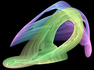
But when these sets (or the motions within them) cannot be easily described as simple combinations (e.g. intersection and union) of fundamental geometric objects (e.g. lines, surfaces, spheres, toroids, manifolds), then the attractor is called a strange attractor.
The final state that a dynamical system evolves towards corresponds to an attracting fixed point of the evolution function for that system, such as the center bottom position of a damped pendulum, the level and flat water line of sloshing water in a glass, or the bottom center of a bowl containing a rolling marble.
In the case of a marble on top of an inverted bowl (a hill), that point at the top of the bowl (hill) is a fixed point (equilibrium), but not an attractor (unstable equilibrium).
In addition, physical dynamic systems with at least one fixed point invariably have multiple fixed points and attractors due to the reality of dynamics in the physical world, including the nonlinear dynamics of stiction, friction, surface roughness, deformation (both elastic and plasticity), and even quantum mechanics.
[6] In the case of a marble on top of an inverted bowl, even if the bowl seems perfectly hemispherical, and the marble's spherical shape, are both much more complex surfaces when examined under a microscope, and their shapes change or deform during contact.
Any physical surface can be seen to have a rough terrain of multiple peaks, valleys, saddle points, ridges, ravines, and plains.
In a discrete-time system, an attractor can take the form of a finite number of points that are visited in sequence.
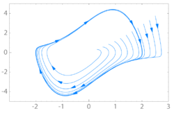
A limit cycle is a periodic orbit of a continuous dynamical system that is isolated.
The difference with the clock pendulum is that there, energy is injected by the escapement mechanism to maintain the cycle.
Such a time series does not have a strict periodicity, but its power spectrum still consists only of sharp lines.
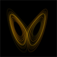
[citation needed] An attractor is called strange if it has a fractal structure, that is if it has non-integer Hausdorff dimension.
If a strange attractor is chaotic, exhibiting sensitive dependence on initial conditions, then any two arbitrarily close alternative initial points on the attractor, after any of various numbers of iterations, will lead to points that are arbitrarily far apart (subject to the confines of the attractor), and after any of various other numbers of iterations will lead to points that are arbitrarily close together.
Strange attractors may also be found in the presence of noise, where they may be shown to support invariant random probability measures of Sinai–Ruelle–Bowen type.
For a stable linear system, every point in the phase space is in the basin of attraction.
gives divergence from all initial points except the vector of zeroes if any eigenvalue of the matrix
is positive; but if all the eigenvalues are negative the vector of zeroes is an attractor whose basin of attraction is the entire phase space.
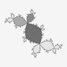
The basins of attraction for the expression's roots are generally not simple—it is not simply that the points nearest one root all map there, giving a basin of attraction consisting of nearby points.
, the following initial conditions are in successive basins of attraction: Newton's method can also be applied to complex functions to find their roots.
The diffusive part of the equation damps higher frequencies and in some cases leads to a global attractor.