Low-pass filter
In optics, high-pass and low-pass may have different meanings, depending on whether referring to the frequency or wavelength of light, since these variables are inversely related.
For this reason, it is a good practice to refer to wavelength filters as short-pass and long-pass to avoid confusion, which would correspond to high-pass and low-pass frequencies.
Low-pass filters provide a smoother form of a signal, removing the short-term fluctuations and leaving the longer-term trend.
[1] In an electronic low-pass RC filter for voltage signals, high frequencies in the input signal are attenuated, but the filter has little attenuation below the cutoff frequency determined by its RC time constant.
Electronic low-pass filters are used on inputs to subwoofers and other types of loudspeakers, to block high pitches that they cannot efficiently reproduce.
Radio transmitters use low-pass filters to block harmonic emissions that might interfere with other communications.
The tone knob on many electric guitars is a low-pass filter used to reduce the amount of treble in the sound.
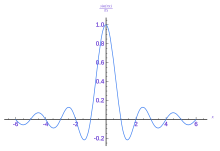
An ideal low-pass filter can be realized mathematically (theoretically) by multiplying a signal by the rectangular function in the frequency domain or, equivalently, convolution with its impulse response, a sinc function, in the time domain.
However, the ideal filter is impossible to realize without also having signals of infinite extent in time, and so generally needs to be approximated for real ongoing signals, because the sinc function's support region extends to all past and future times.
Truncating an ideal low-pass filter result in ringing artifacts via the Gibbs phenomenon, which can be reduced or worsened by the choice of windowing function.
Design and choice of real filters involves understanding and minimizing these artifacts.
The most common way to characterize the frequency response of a circuit is to find its Laplace transform[6] transfer function,
we get A discrete difference equation is easily obtained by sampling the step input response above at regular intervals of
, this model approximates the input signal as a series of step functions with duration
The error produced from time variant inputs is difficult to quantify[citation needed] but decreases as
For simplicity, assume that samples of the input and output are taken at evenly spaced points in time separated by
Making these substitutions, Rearranging terms gives the recurrence relation That is, this discrete-time implementation of a simple RC low-pass filter is the exponentially weighted moving average By definition, the smoothing factor is within the range
The expression for α yields the equivalent time constant RC in terms of the sampling period
Only O(n log(n)) operations are required compared to O(n2) for the time domain filtering algorithm.
This can also sometimes be done in real time, where the signal is delayed long enough to perform the Fourier transformation on shorter, overlapping blocks.
In all cases, at the cutoff frequency, the filter attenuates the input power by half or 3 dB.
Continuous-time filters can also be described in terms of the Laplace transform of their impulse response, in a way that lets all characteristics of the filter be easily analyzed by considering the pattern of poles and zeros of the Laplace transform in the complex plane.
For example, a first-order low-pass filter can be described by the continuous time transfer function, in the Laplace domain, as: where H is the transfer function, s is the Laplace transform variable (complex angular frequency), τ is the filter time constant,
The capacitor exhibits reactance, and blocks low-frequency signals, forcing them through the load instead.
At higher frequencies, the reactance drops, and the capacitor effectively functions as a short circuit.
A first-order RL circuit is one of the simplest analogue infinite impulse response electronic filters.
The RLC part of the name is due to those letters being the usual electrical symbols for resistance, inductance, and capacitance, respectively.
The main difference that the presence of the resistor makes is that any oscillation induced in the circuit will die away over time if it is not kept going by a source.
Some resistance is unavoidable in real circuits, even if a resistor is not specifically included as a component.
In the operational amplifier circuit shown in the figure, the cutoff frequency (in hertz) is defined as: or equivalently (in radians per second): The gain in the passband is −R2/R1, and the stopband drops off at −6 dB per octave (that is −20 dB per decade) as it is a first-order filter.