Resonance
When this happens, the object or system absorbs energy from the external force and starts vibrating with a larger amplitude.
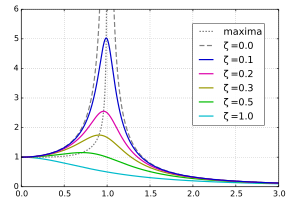
Peaks in the gain at certain frequencies correspond to resonances, where the amplitude of the measured output's oscillations are disproportionately large.
An RLC circuit is used to illustrate connections between resonance and a system's transfer function, frequency response, poles, and zeroes.
Building off the RLC circuit example, these connections for higher-order linear systems with multiple inputs and outputs are generalized.
It is possible to write the steady-state solution for x(t) as a function proportional to the driving force with an induced phase change φ, where
For other driven, damped harmonic oscillators whose equations of motion do not look exactly like the mass on a spring example, the resonant frequency remains
Evaluating H(s) along the imaginary axis s = iω, the transfer function describes the frequency response of this circuit.
The frequency that is filtered out corresponds exactly to the zeroes of the transfer function, which were shown in Equation (7) and were on the imaginary axis.
Specifically, these examples illustrate: The next section extends these concepts to resonance in a general linear system.
For example, in state-space representation a third order linear time-invariant system with three inputs and two outputs might be written as
Peaks in the gain at certain frequencies correspond to resonances between that transfer function's input and output, assuming the system is stable.
As the number of coupled harmonic oscillators increases, the time it takes to transfer energy from one to the next becomes significant.
For example, the string of a guitar or the surface of water in a bowl can be modeled as a continuum of small coupled oscillators and waves can travel along them.
In many cases these systems have the potential to resonate at certain frequencies, forming standing waves with large-amplitude oscillations at fixed positions.
Resonance in the form of standing waves underlies many familiar phenomena, such as the sound produced by musical instruments, electromagnetic cavities used in lasers and microwave ovens, and energy levels of atoms.
It may cause violent swaying motions and even catastrophic failure in improperly constructed structures including bridges, buildings, trains, and aircraft.
Avoiding resonance disasters is a major concern in every building, tower, and bridge construction project.
Buildings in seismic zones are often constructed to take into account the oscillating frequencies of expected ground motion.
Resonance in circuits are used for both transmitting and receiving wireless communications such as television, cell phones and radio.
Light confined in the cavity reflects multiple times producing standing waves for certain resonant frequencies.
In most cases, this results in an unstable interaction, in which the bodies exchange momentum and shift orbits until the resonance no longer exists.
A key feature of NMR is that the resonant frequency of a particular substance is directly proportional to the strength of the applied magnetic field.
The Mössbauer effect is the resonant and recoil-free emission and absorption of gamma ray photons by atoms bound in a solid form.
A column of soldiers marching in regular step on a narrow and structurally flexible bridge can set it into dangerously large amplitude oscillations.
On April 12, 1831, the Broughton Suspension Bridge near Salford, England collapsed while a group of British soldiers were marching across.
Several early suspension bridges in Europe and United States were destroyed by structural resonance induced by modest winds.
The collapse of the Tacoma Narrows Bridge on 7 November 1940 is characterized in physics as a classic example of resonance.
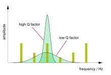
In electrical resonance, a high-Q circuit in a radio receiver is more difficult to tune, but has greater selectivity, and so would be better at filtering out signals from other stations.
This is a Lorentzian function, or Cauchy distribution, and this response is found in many physical situations involving resonant systems.
In radio engineering and electronics engineering, this approximate symmetric response is known as the universal resonance curve, a concept introduced by Frederick E. Terman in 1932 to simplify the approximate analysis of radio circuits with a range of center frequencies and Q values.