Optical transfer function
As a Fourier transform, the OTF is generally complex-valued; however, it is real-valued in the common case of a PSF that is symmetric about its center.
Its transfer function decreases approximately gradually with spatial frequency until it reaches the diffraction-limit, in this case at 500 cycles per millimeter or a period of 2 μm.
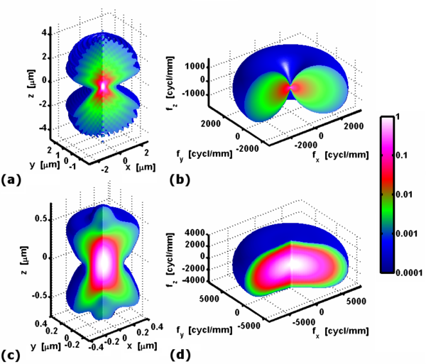
The impulse response of a well-focused optical system is a three-dimensional intensity distribution with a maximum at the focal plane, and could thus be measured by recording a stack of images while displacing the detector axially.
Generally, the optical transfer function depends on factors such as the spectrum and polarization of the emitted light and the position of the point source.
When significant variation occurs, the optical transfer function may be calculated for a set of representative positions or colors.
Note that sometimes the optical transfer function is given in units of the object or sample space, observation angle, film width, or normalized to the theoretical maximum.
As explained by the Nyquist–Shannon sampling theorem, to match the optical resolution of the given example, the pixels of each color channel should be separated by 1 micrometer, half the period of 500 cycles per millimeter.
While optical resolution, as commonly used with reference to camera systems, describes only the number of pixels in an image, and hence the potential to show fine detail, the transfer function describes the ability of adjacent pixels to change from black to white in response to patterns of varying spatial frequency, and hence the actual capability to show fine detail, whether with full or reduced contrast.
Taking the example of a current high definition (HD) video system, with 1920 by 1080 pixels, the Nyquist theorem states that it should be possible, in a perfect system, to resolve fully (with true black to white transitions) a total of 1920 black and white alternating lines combined, otherwise referred to as a spatial frequency of 1920/2=960 line pairs per picture width, or 960 cycles per picture width, (definitions in terms of cycles per unit angle or per mm are also possible but generally less clear when dealing with cameras and more appropriate to telescopes etc.).
In practice, this is far from the case, and spatial frequencies that approach the Nyquist rate will generally be reproduced with decreasing amplitude, so that fine detail, though it can be seen, is greatly reduced in contrast.
Ideal systems such as in the examples here are readily calculated numerically using software such as Julia, GNU Octave or Matlab, and in some specific cases even analytically.
The optical transfer function of such a system can thus be calculated geometrically from the intersecting area between two identical disks at a distance of
At high numerical apertures such as those found in microscopy, it is important to consider the vectorial nature of the fields that carry light.
When the aberrations can be assumed to be spatially invariant, alternative patterns can be used to determine the optical transfer function such as lines and edges.
Such extended objects illuminate more pixels in the image, and can improve the measurement accuracy due to the larger signal-to-noise ratio.
The optical transfer function is in this case calculated as the two-dimensional discrete Fourier transform of the image and divided by that of the extended object.
It can be found directly from an ideal line approximation provided by a slit test target or it can be derived from the edge spread function, discussed in the next sub section.
Although the measurement images obtained with this technique illuminate a large area of the camera, this mainly benefits the accuracy at low spatial frequencies.
As shown in the right hand figure, an operator defines a box area encompassing the edge of a knife-edge test target image back-illuminated by a black body.
In case it is more practical to measure the edge spread function, one can determine the line spread function as follows: Typically the ESF is only known at discrete points, so the LSF is numerically approximated using the finite difference: where: Although 'sharpness' is often judged on grid patterns of alternate black and white lines, it should strictly be measured using a sine-wave variation from black to white (a blurred version of the usual pattern).
A square wave test chart will therefore show optimistic results (better resolution of high spatial frequencies than is actually achieved).
A major factor is usually the impossibility of making the perfect 'brick wall' optical filter (often realized as a 'phase plate' or a lens with specific blurring properties in digital cameras and video camcorders).
The only way in practice to approach the theoretical sharpness possible in a digital imaging system such as a camera is to use more pixels in the camera sensor than samples in the final image, and 'downconvert' or 'interpolate' using special digital processing which cuts off high frequencies above the Nyquist rate to avoid aliasing whilst maintaining a reasonably flat MTF up to that frequency.
The only theoretically correct way to interpolate or downconvert is by use of a steep low-pass spatial filter, realized by convolution with a two-dimensional sin(x)/x weighting function which requires powerful processing.
However much we raise the number of pixels used in cameras, this will always remain true in absence of a perfect optical spatial filter.
Because of the problem of maintaining a high contrast MTF, broadcasters like the BBC did for a long time consider maintaining standard definition television, but improving its quality by shooting and viewing with many more pixels (though as previously mentioned, such a system, though impressive, does ultimately lack the very fine detail which, though attenuated, enhances the effect of true HD viewing).
[12] There has recently been a shift towards the use of large image format digital single-lens reflex cameras driven by the need for low-light sensitivity and narrow depth of field effects.
Such cameras produce very impressive results, and appear to be leading the way in video production towards large-format downconversion with digital filtering becoming the standard approach to the realization of a flat MTF with true freedom from aliasing.
The optical contrast reduction can be partially reversed by digitally amplifying spatial frequencies selectively before display or further processing.
Although more advanced digital image restoration procedures exist, the Wiener deconvolution algorithm is often used for its simplicity and efficiency.