Nonlinear dimensionality reduction
Nonlinear dimensionality reduction, also known as manifold learning, is any of various related techniques that aim to project high-dimensional data, potentially existing across non-linear manifolds which cannot be adequately captured by linear decomposition methods, onto lower-dimensional latent manifolds, with the goal of either visualizing the data in the low-dimensional space, or learning the mapping (either from the high-dimensional space to the low-dimensional embedding or vice versa) itself.
High dimensional data can be hard for machines to work with, requiring significant time and space for analysis.
Reducing the dimensionality of a data set, while keep its essential features relatively intact, can make algorithms more efficient and allow analysts to visualize trends and patterns.
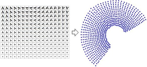
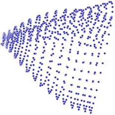
By comparison, if principal component analysis, which is a linear dimensionality reduction algorithm, is used to reduce this same dataset into two dimensions, the resulting values are not so well organized.
This demonstrates that the high-dimensional vectors (each representing a letter 'A') that sample this manifold vary in a non-linear manner.
Invariant manifolds are of general interest for model order reduction in dynamical systems.
In particular, if there is an attracting invariant manifold in the phase space, nearby trajectories will converge onto it and stay on it indefinitely, rendering it a candidate for dimensionality reduction of the dynamical system.
[3] Active research in NLDR seeks to unfold the observation manifolds associated with dynamical systems to develop modeling techniques.
The objective function includes a quality of data approximation and some penalty terms for the bending of the manifold.
[14] This technique relies on the basic assumption that the data lies in a low-dimensional manifold in a high-dimensional space.
[15] This algorithm cannot embed out-of-sample points, but techniques based on Reproducing kernel Hilbert space regularization exist for adding this capability.
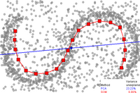
Traditional techniques like principal component analysis do not consider the intrinsic geometry of the data.
The graph thus generated can be considered as a discrete approximation of the low-dimensional manifold in the high-dimensional space.
The original point is approximately reconstructed by a linear combination, given by the weight matrix Wij, of its neighbors.
The creators of this regularised variant are also the authors of Local Tangent Space Alignment (LTSA), which is implicit in the MLLE formulation when realising that the global optimisation of the orthogonal projections of each weight vector, in-essence, aligns the local tangent spaces of every data point.
Its initial step, like Isomap and Locally Linear Embedding, is finding the k-nearest neighbors of every point.
Thus, the network must learn to encode the vector into a small number of dimensions and then decode it back into the original space.
The model is defined probabilistically and the latent variables are then marginalized and parameters are obtained by maximizing the likelihood.
It was originally proposed for visualization of high dimensional data but has been extended to construct a shared manifold model between two observation spaces.
The algorithm computes the probability that pairs of datapoints in the high-dimensional space are related, and then chooses low-dimensional embeddings which produce a similar distribution.
Relational perspective map was inspired by a physical model in which positively charged particles move freely on the surface of a ball.
[30] CDA[29] trains a self-organizing neural network to fit the manifold and seeks to preserve geodesic distances in its embedding.
The methods solves for a smooth time indexed vector field such that flows along the field which start at the data points will end at a lower-dimensional linear subspace, thereby attempting to preserve pairwise differences under both the forward and inverse mapping.
By learning projections from each original space to the shared manifold, correspondences are recovered and knowledge from one domain can be transferred to another.
The underlying assumption of diffusion map is that the high-dimensional data lies on a low-dimensional manifold of dimension
[36] Nonlinear PCA (NLPCA) uses backpropagation to train a multi-layer perceptron (MLP) to fit to a manifold.
Data-driven high-dimensional scaling (DD-HDS)[38] is closely related to Sammon's mapping and curvilinear component analysis except that (1) it simultaneously penalizes false neighborhoods and tears by focusing on small distances in both original and output space, and that (2) it accounts for concentration of measure phenomenon by adapting the weighting function to the distance distribution.
Like other algorithms, it computes the k-nearest neighbors and tries to seek an embedding that preserves relationships in local neighborhoods.
Uniform manifold approximation and projection (UMAP) is a nonlinear dimensionality reduction technique.
The variations tend to be differences in how the proximity data is computed; for example, isomap, locally linear embeddings, maximum variance unfolding, and Sammon mapping (which is not in fact a mapping) are examples of metric multidimensional scaling methods.