Linear discriminant analysis

LDA works when the measurements made on independent variables for each observation are continuous quantities.

When dealing with categorical independent variables, the equivalent technique is discriminant correspondence analysis.

[8] In simple terms, discriminant function analysis is classification - the act of distributing things into groups, classes or categories of the same type.

The original dichotomous discriminant analysis was developed by Sir Ronald Fisher in 1936.

Discriminant function analysis is useful in determining whether a set of variables is effective in predicting category membership.

(also called features, attributes, variables or measurements) for each sample of an object or event with known class

LDA instead makes the additional simplifying homoscedasticity assumption (i.e. that the class covariances are identical, so

The analysis is quite sensitive to outliers and the size of the smallest group must be larger than the number of predictor variables.

[14] Each function is given a discriminant score[clarification needed] to determine how well it predicts group placement.

[10][8] The eigenvalue can be viewed as a ratio of SSbetween and SSwithin as in ANOVA when the dependent variable is the discriminant function, and the groups are the levels of the IV[clarification needed].

[10] Another popular measure of effect size is the percent of variance[clarification needed] for each function.

[10]Kappa normalizes across all categorizes rather than biased by a significantly good or poorly performing classes.

[19] The terms Fisher's linear discriminant and LDA are often used interchangeably, although Fisher's original article[2] actually describes a slightly different discriminant, which does not make some of the assumptions of LDA such as normally distributed classes or equal class covariances.

can be found explicitly: Otsu's method is related to Fisher's linear discriminant, and was created to binarize the histogram of pixels in a grayscale image by optimally picking the black/white threshold that minimizes intra-class variance and maximizes inter-class variance within/between grayscales assigned to black and white pixel classes.

is diagonalizable, the variability between features will be contained in the subspace spanned by the eigenvectors corresponding to the C − 1 largest eigenvalues (since

The eigenvectors corresponding to the smaller eigenvalues will tend to be very sensitive to the exact choice of training data, and it is often necessary to use regularisation as described in the next section.

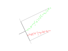
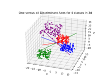
A common example of this is "one against the rest" where the points from one class are put in one group, and everything else in the other, and then LDA applied.

For example, in many real-time applications such as mobile robotics or on-line face recognition, it is important to update the extracted LDA features as soon as new observations are available.

[24] Later, Aliyari et al. derived fast incremental algorithms to update the LDA features by observing the new samples.

[25] Another strategy to deal with small sample size is to use a shrinkage estimator of the covariance matrix, which can be expressed mathematically as where

In marketing, discriminant analysis was once often used to determine the factors which distinguish different types of customers and/or products on the basis of surveys or other forms of collected data.

Then results of clinical and laboratory analyses are studied to reveal statistically different variables in these groups.

Using these variables, discriminant functions are built to classify disease severity in future patients.

[32] In biology, similar principles are used in order to classify and define groups of different biological objects, for example, to define phage types of Salmonella enteritidis based on Fourier transform infrared spectra,[33] to detect animal source of Escherichia coli studying its virulence factors[34] etc.

[35] Discriminant function analysis is very similar to logistic regression, and both can be used to answer the same research questions.

[36] Unlike logistic regression, discriminant analysis can be used with small sample sizes.

It has been shown that when sample sizes are equal, and homogeneity of variance/covariance holds, discriminant analysis is more accurate.

[8] Despite all these advantages, logistic regression has none-the-less become the common choice, since the assumptions of discriminant analysis are rarely met.

[39] In particular, such theorems are proven for log-concave distributions including multidimensional normal distribution (the proof is based on the concentration inequalities for log-concave measures[40]) and for product measures on a multidimensional cube (this is proven using Talagrand's concentration inequality for product probability spaces).

Data separability by classical linear discriminants simplifies the problem of error correction for artificial intelligence systems in high dimension.