Proportional–integral–derivative controller

The PID controller adjusts the engine's power output to restore the vehicle to its desired speed, doing so efficiently with minimal delay and overshoot.

The theoretical foundation of PID controllers dates back to the early 1920s with the development of automatic steering systems for ships.

Approximate values of constants can usually be initially entered knowing the type of application, but they are normally refined, or tuned, by introducing a setpoint change and observing the system response.

PI controllers are fairly common in applications where derivative action would be sensitive to measurement noise, but the integral term is often needed for the system to reach its target value.

[3][4] With the invention of the low-pressure stationary steam engine there was a need for automatic speed control, and James Watt's self-designed "conical pendulum" governor, a set of revolving steel balls attached to a vertical spindle by link arms, came to be an industry standard.

He explored the mathematical basis for control stability, and progressed a good way towards a solution, but made an appeal for mathematicians to examine the problem.

[6][5] The problem was examined further in 1874 by Edward Routh, Charles Sturm, and in 1895, Adolf Hurwitz, all of whom contributed to the establishment of control stability criteria.

The pendulum added what is now known as derivative control, which damped the oscillations by detecting the torpedo dive/climb angle and thereby the rate-of-change of depth.

[10] Minorsky was researching and designing automatic ship steering for the US Navy and based his analysis on observations of a helmsman.

They were simple low maintenance devices that operated well in harsh industrial environments and did not present explosion risks in hazardous locations.

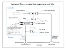
By measuring the position (PV), and subtracting it from the setpoint (SP), the error (e) is found, and from it the controller calculates how much electric current to supply to the motor (MV).

The PID control scheme is named after its three correcting terms, whose sum constitutes the manipulated variable (MV).

The integral in a PID controller is the sum of the instantaneous error over time and gives the accumulated offset that should have been corrected previously.

Derivative action is seldom used in practice though – by one estimate in only 25% of deployed controllers [citation needed] – because of its variable impact on system stability in real-world applications.

Designing and tuning a PID controller appears to be conceptually intuitive, but can be hard in practice, if multiple (and often conflicting) objectives, such as short transient and high stability, are to be achieved.

Usually, initial designs need to be adjusted repeatedly through computer simulations until the closed-loop system performs or compromises as desired.

Similar to the Ziegler–Nichols method, a set of tuning parameters were developed to yield a closed-loop response with a decay ratio of

Published in 1984 by Karl Johan Åström and Tore Hägglund,[25] the relay method temporarily operates the process using bang-bang control and measures the resultant oscillations.

Another approach calculates initial values via the Ziegler–Nichols method, and uses a numerical optimization technique to find better PID coefficients.

Alternatively, PIDs can be modified in more minor ways, such as by changing the parameters (either gain scheduling in different use cases or adaptively modifying them based on performance), improving measurement (higher sampling rate, precision, and accuracy, and low-pass filtering if necessary), or cascading multiple PID controllers.

A non-linear valve, for instance, in a flow control application, will result in variable loop sensitivity, requiring dampened action to prevent instability.

A problem with the derivative term is that it amplifies higher frequency measurement or process noise that can cause large amounts of change in the output.

This overshoot can be avoided by freezing of the integral function after the opening of the door for the time the control loop typically needs to reheat the furnace.

A PI controller can be modelled easily in software such as Simulink or Xcos using a "flow chart" box involving Laplace operators: where Setting a value for

The proportional and derivative terms can produce excessive movement in the output when a system is subjected to an instantaneous step increase in the error, such as a large setpoint change.

PID controllers are often implemented with a "bumpless" initialization feature that recalculates the integral accumulator term to maintain a consistent process output through parameter changes.

The outer PID controller has a long time constant – all the water in the tank needs to heat up or cool down.

However, it is also the form where the parameters have the weakest relationship to physical behaviors and is generally reserved for theoretical treatment of the PID controller.

temperature regulation using a motor controlling a valve), Kp, Ki and Kd may be corrected by a unit conversion factor.

In the real world, this is D-to-A converted and passed into the process under control as the manipulated variable (MV).