Phillips curve

Paul Samuelson and Robert Solow made the connection explicit and subsequently Milton Friedman[2] and Edmund Phelps[3][4] put the theoretical structure in place.

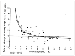
[11] In the paper Phillips describes how he observed an inverse relationship between money wage changes and unemployment in the British economy over the period examined.

[13] In the years following Phillips' 1958 paper, many economists in advanced industrial countries believed that his results showed a permanently stable relationship between inflation and unemployment.

[citation needed] Economist James Forder disputes this history and argues that it is a 'Phillips curve myth' invented in the 1970s.

[14] Since 1974, seven Nobel Prizes have been given to economists for, among other things, work critical of some variations of the Phillips curve.

It would be wrong, though, to think that our Figure 2 menu that related obtainable price and unemployment behavior will maintain its same shape in the longer run.

Work by George Akerlof, William Dickens, and George Perry,[16] implies that if inflation is reduced from two to zero percent, unemployment will be permanently increased by 1.5 percent because workers have a higher tolerance for real wage cuts than nominal ones.

The theory has several names, with some variation in its details, but all modern versions distinguish between short-run and long-run effects on unemployment.

This is because in the short run, there is generally an inverse relationship between inflation and the unemployment rate; as illustrated in the downward sloping short-run Phillips curve.

In the long run, this implies that monetary policy cannot affect unemployment, which adjusts back to its "natural rate", also called the "NAIRU".

[19] An equation like the expectations-augmented Phillips curve also appears in many recent New Keynesian dynamic stochastic general equilibrium models.

As Keynes mentioned: "A Government has to remember, however, that even if a tax is not prohibited it may be unprofitable, and that a medium, rather than an extreme, imposition will yield the greatest gain".

The focus is on only production workers' money wages, because (as discussed below) these costs are crucial to pricing decisions by the firms.

A major one is that money wages are set by bilateral negotiations under partial bilateral monopoly: as the unemployment rate rises, all else constant worker bargaining power falls, so that workers are less able to increase their wages in the face of employer resistance.

In the long run, it is assumed, inflationary expectations catch up with and equal actual inflation so that gP = gPex.

This logic goes further if λ is equal to unity, i.e., if workers are able to protect their wages completely from expected inflation, even in the short run.

Now, the Triangle Model equation becomes: If we further assume (as seems reasonable) that there are no long-term supply shocks, this can be simplified to become: All of the assumptions imply that in the long run, there is only one possible unemployment rate, U* at any one time.

One important place to look is at the determination of the mark-up, M. The Phillips curve equation can be derived from the (short-run) Lucas aggregate supply function.

This differs from other views of the Phillips curve, in which the failure to attain the "natural" level of output can be due to the imperfection or incompleteness of markets, the stickiness of prices, and the like.

To the "new Classical" followers of Lucas, markets are presumed to be perfect and always attain equilibrium (given inflationary expectations).

In the 1970s, new theories, such as rational expectations and the NAIRU (non-accelerating inflation rate of unemployment) arose to explain how stagflation could occur.

Milton Friedman in 1976 and Edmund Phelps in 2006 won the Nobel Prize in Economics in part for this work.

[26] [27] However, the expectations argument was in fact very widely understood (albeit not formally) before Friedman's and Phelps's work on it.

This, in turn, suggested that the short-run period was so short that it was non-existent: any effort to reduce unemployment below the NAIRU, for example, would immediately cause inflationary expectations to rise and thus imply that the policy would fail.

Unemployment would never deviate from the NAIRU except due to random and transitory mistakes in developing expectations about future inflation rates.

In the late 1990s, the actual unemployment rate fell below 4% of the labor force, much lower than almost all estimates of the NAIRU.

Furthermore, the concept of rational expectations had become subject to much doubt when it became clear that the main assumption of models based on it was that there exists a single (unique) equilibrium in the economy that is set ahead of time, determined independently of demand conditions.

When an inflationary surprise occurs, workers are fooled into accepting lower pay because they do not see the fall in real wages right away.

This information asymmetry and a special pattern of flexibility of prices and wages are both necessary if one wants to maintain the mechanism told by Friedman.

[29] Robert J. Gordon of Northwestern University has analyzed the Phillips curve to produce what he calls the triangle model, in which the actual inflation rate is determined by the sum of The last reflects inflationary expectations and the price/wage spiral.