Lotka–Volterra equations

This, in turn, implies that the generations of both the predator and prey are continually overlapping.

[1] The Lotka–Volterra system of equations is an example of a Kolmogorov population model (not to be confused with the better known Kolmogorov equations),[2][3][4] which is a more general framework that can model the dynamics of ecological systems with predator–prey interactions, competition, disease, and mutualism.

The term γy represents the loss rate of the predators due to either natural death or emigration; it leads to an exponential decay in the absence of prey.

Nevertheless, the Lotka–Volterra model shows two important properties of predator and prey populations and these properties often extend to variants of the model in which these assumptions are relaxed: Firstly, the dynamics of predator and prey populations have a tendency to oscillate.

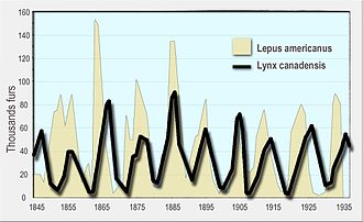
Fluctuating numbers of predators and prey have been observed in natural populations, such as the lynx and snowshoe hare data of the Hudson's Bay Company[6] and the moose and wolf populations in Isle Royale National Park.

The addition of iron typically leads to a short bloom in phytoplankton, which is quickly consumed by other organisms (such as small fish or zooplankton) and limits the effect of enrichment mainly to increased predator density, which in turn limits the carbon sequestration.

[10][11] It can be used to describe the dynamics in a market with several competitors, complementary platforms and products, a sharing economy, and more.

The Lotka–Volterra predator–prey model was initially proposed by Alfred J. Lotka in the theory of autocatalytic chemical reactions in 1910.

[12][13] This was effectively the logistic equation,[14] originally derived by Pierre François Verhulst.

[17] The same set of equations was published in 1926 by Vito Volterra, a mathematician and physicist, who had become interested in mathematical biology.

[13][18][19] Volterra's enquiry was inspired through his interactions with the marine biologist Umberto D'Ancona, who was courting his daughter at the time and later was to become his son-in-law.

Volterra developed his model to explain D'Ancona's observation and did this independently from Alfred Lotka.

[21] Both the Lotka–Volterra and Rosenzweig–MacArthur models have been used to explain the dynamics of natural populations of predators and prey.

[23] The Lotka–Volterra equations have a long history of use in economic theory; their initial application is commonly credited to Richard Goodwin in 1965[24] or 1967.

These solutions do not have a simple expression in terms of the usual trigonometric functions, although they are quite tractable.

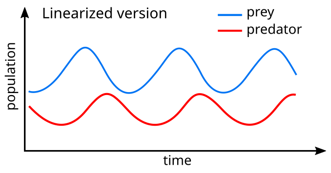
A linearization of the equations yields a solution similar to simple harmonic motion[30] with the population of predators trailing that of prey by 90° in the cycle.

Suppose there are two species of animals, a rabbit (prey) and a fox (predator).

It is amenable to separation of variables: integrating yields the implicit relationship where V is a constant quantity depending on the initial conditions and conserved on each curve.

An aside: These graphs illustrate a serious potential limitation in the application as a biological model: for this specific choice of parameters, in each cycle, the rabbit population is reduced to extremely low numbers, yet recovers (while the fox population remains sizeable at the lowest rabbit density).

In real-life situations, however, chance fluctuations of the discrete numbers of individuals might cause the rabbits to actually go extinct, and, by consequence, the foxes as well.

is conserved over time, it plays role of a Hamiltonian function of the system.

Circles represent prey and predator initial conditions from x = y = 0.9 to 1.8, in steps of 0.1.

In the model system, the predators thrive when prey is plentiful but, ultimately, outstrip their food supply and decline.

The second solution represents a fixed point at which both populations sustain their current, non-zero numbers, and, in the simplified model, do so indefinitely.

The levels of population at which this equilibrium is achieved depend on the chosen values of the parameters α, β, γ, and δ.

The stability of the fixed point at the origin can be determined by performing a linearization using partial derivatives.

(In fact, this could only occur if the prey were artificially completely eradicated, causing the predators to die of starvation.

If the predators were eradicated, the prey population would grow without bound in this simple model.)

As the eigenvalues are both purely imaginary and conjugate to each other, this fixed point must either be a center for closed orbits in the local vicinity or an attractive or repulsive spiral.

As illustrated in the circulating oscillations in the figure above, the level curves are closed orbits surrounding the fixed point: the levels of the predator and prey populations cycle and oscillate without damping around the fixed point with frequency