The idea that a form of turbulence might be possible in a superfluid via the quantized vortex lines was first suggested by Richard Feynman.
The A-phase is strongly anisotropic, and although it has very interesting hydrodynamic properties, turbulence experiments have been performed almost exclusively in the B-phase.
[4] Although in atomic condensates there is not as much experimental evidence for turbulence as in Helium, experiments have been performed with rubidium, sodium, caesium, lithium and other elements.
Superfluidity arises as a consequence of the dispersion relation of elementary excitations, and fluids that exhibit this behaviour flow without viscosity.
The property of quantized circulation arises as a consequence of the existence and uniqueness of a complex macroscopic wavefunction
, which affects the vorticity (local rotation) in a very profound way, making it crucial for quantum turbulence.
, Stokes theorem holds, and the circulation vanishes, as the velocity can be expressed as the gradient of the phase.
This leads to the idea of the Rankine vortex as shown in fig 2, which combines solid body rotation for small
Many similarities can be drawn with vortices in classical fluids, for example the fact that vortex lines obey the classical Kelvin circulation theorem: the circulation is conserved and the vortex lines must terminate at boundaries or exist in the shape of closed loops.
Vortices in quantum fluids support Kelvin waves, which are helical perturbations of a vortex line away from its straight configuration that rotate at an angular velocity
For atomic gases at non-zero temperatures, a fraction of the atoms are not part of the condensate, but rather form a rarefied (large free mean path) thermal cloud that co-exist with the condensate (which, in the first approximation, can be identified with the superfluid component).
This forms the basis of Tisza's and Landau's two-fluid theory describing helium II as the mixture of co-penetrating superfluid and normal fluid components, with a total density dictated by the equation
The turbulence of classical fluids is an everyday phenomenon, which can be readily observed in the flow of a stream or river as was first done by Leonardo da Vinci in his famous sketches.
Such turbulence can be created inside of a wind tunnel, for example a channel with air flow propelled by a fan from one side to the other.
A statistically steady state ensures that the main properties of the flow stabilises even though they fluctuate locally.
Due to presence of viscosity, without the continuous supply of energy the turbulence of the flow will decay because of frictional forces.
The notion of an energy cascade, where an energy transfer takes place from large scale vortices to smaller scale vortices, which eventually lead to viscous dissipation, was memorably noted by Lewis Fry Richardson.
In a pure superfluid, there is no normal component to carry the entropy of the system and therefore the fluid flows without viscosity, resulting in the lack of a dissipation scale
) can be introduced by replacing the kinematic viscosity in the Kolmogorov length scale with the quantum of circulation
, a small polarisation of the vortex lines allows the stretching required to sustain a Kolmogorov energy cascade.
Experiments have been performed in superfluid Helium II to create turbulence, that behave according to the Kolmogorov cascade.
For higher temperatures, the existence of the normal fluid component leads to the presence of viscous forces and eventual heat dissipation which warms the system.
[11] For temperatures in the zero limit, the undamped Kelvin waves result in more kinks appearing in the shapes of the vortices.
Vinen turbulence can be generated in a quantum fluid by the injection of vortex rings into the system, which has been observed both numerically and experimentally.
The partial polarization contributes strongly to the amount of non-local interactions between the vortex lines, which can be seen in the figure.
As a result of these properties Vinen turbulence appears as an almost completely random flow with a very weak or negligible energy cascade.
Stemming from the different signatures, Kolmogorov and Vinen turbulence follow power laws relating to their temporal decay.
Quantum turbulence is characterised by a disordered tangle of discrete (individual) vortex lines.
(the length of vortex lines per unit volume based on detecting the second sound attenuation.
Quantum turbulence can be detected in 3He-B in two ways: nuclear magnetic resonance (NMR) [41] and by Andreev scattering of thermal quasiparticles.
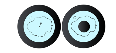
Fig 1. The schematic diagram of a fluid (blue) in a cylindrical container. Left: The curve
traces out a closed path in a simply connected region. The path can be shrunk down to the point
, and therefore Stokes theorem can be applied. For a quantum fluid, this indicates that the circulation vanishes. Right: The curve
traces out a closed path in a multiply-connected region (i.e. with holes). The path cannot be shrunk down due to the hole, and therefore Stokes theorem does not hold, leading to a non-zero, quantized circulation. For a quantum fluid, this suggests that vortex structures act like 'holes'.
Fig 2. Left: Simple schematic of a straight vortex line in 3-dimensional space, with positive circulation. Middle: Azimuthal velocity against the radius. (i) shows the fluid speed of a solid-body rotation. (ii) shows the fluid speed of a vortex in both classical and quantum fluids. (iii) a combination of (i) and (ii) to form a Rankine vortex model for a tornado with core of size
. Right: Number density against radius of a quantum fluid with vortex
. Density depletion can be observed for a small radius
. The quantity
represents the density of the fluid sufficiently far away from the vortex core
.
Fig 3. Left: Schematic of a vortex ring of radius
moving at a speed
. Middle: 3-dimensional schematic of a quantum vortex ring. The velocity of the ring is generated by the ring itself, which propels itself at a velocity that is inversely proportional to the radius of the ring. The thickness of the ring is greatly exaggerated for the purpose of being able to view the torus-like shape. In reality, for helium II the thickness is approximately
. Right: The velocity profile of the vortex ring against its size. An inverse relationship can be viewed. This suggests that smaller rings move at a much faster speed, while larger rings move at a much slower speed.
Fig 4. Left: Schematic of a Kelvin wave with amplitude
and wavelength
. Right: A straight vortex configuration that has been perturbed into a bent vortex configuration.
Fig 5. Schematic of vortex reconnection of two vortices. The arrows on the vortices represent the direction of the vorticity in the vortex line. Left: Before the reconnection. Middle: The vortex reconnection is taking place. Right: after the reconnection.
Fig 6. Schematic of a cylindrical container rotating at a speed of
, forming a vortex lattice of six straight vortex lines.
Fig 7. Component fractions plotted against the temperature, displaying the mixture of normal fluid and superfluid in helium II, where
is the superfluid fraction, and
is the normal fluid fraction. For temperatures above the critical temperature, the normal fluid makes up the whole fluid.
Fig 8. Schematic diagram of the Kolmogorov energy cascade inside of a wind tunnel. The injection of air occurs at
where
is the size of the wind tunnel. The quantity
, the Kolmogorov wavenumber, is the value in k-space associated to the
Kolmogorov length scale
, the point at which the turbulent kinetic energy is dissipated into heat.
Fig 9a. Numerically simulated vortex tangle representing Kolmogorov quantum turbulence. The thin lines represent vortex lines inside of a cubic container. The colorbar
[
7
]
[
8
]
represents the amount of non-local interaction, i.e. the amount by how much a section of the vortex line is affected by the other vortex lines surrounding it. (Credit AW Baggaley)
Fig 9. Schematic diagram of the energy spectrum for Kolmogorov turbulence at very small temperatures. The
energy cascade is present for large length scales, and a Kelvin wave cascade can be observed for very small length scales which undergoes sound emission. A bottleneck pile up occurs around the quantum length scale
.
[
9
]
Fig 9b. Numerically simulated vortex tangle representing vinen quantum turbulence. The thin lines represent vortex lines inside of a cubic container. The colorbar
[
7
]
[
8
]
represents the amount of non-local interaction, i.e. the amount by how much a section of the vortex line is affected by the other vortex lines surrounding it. (Credit AW Baggaley)
Fig 10. Schematic diagram of the energy spectrum for vinen turbulence. A
regime can be observed for very large wavenumbers, with the peak of the energy spectrum occurring at the wavenumber
associated to the quantum length scale
. The green line represents a
regime for comparison.
Fig 11. A simulated vortex tangle representing quantum turbulence in a cubic volume and showing the quantized vortices