Rayleigh fading
Rayleigh fading is a statistical model for the effect of a propagation environment on a radio signal, such as that used by wireless devices.
Rayleigh fading models assume that the magnitude of a signal that has passed through such a transmission medium (also called a communication channel) will vary randomly, or fade, according to a Rayleigh distribution — the radial component of the sum of two uncorrelated Gaussian random variables.
[1][2] Rayleigh fading is most applicable when there is no dominant propagation along a line of sight between the transmitter and receiver.
Rayleigh fading is a reasonable model when there are many objects in the environment that scatter the radio signal before it arrives at the receiver.
The central limit theorem holds that, if there is sufficiently much scatter, the channel impulse response will be well-modelled as a Gaussian process irrespective of the distribution of the individual components.
If there is no dominant component to the scatter, then such a process will have zero mean and phase evenly distributed between 0 and 2π radians.
Often, the gain and phase elements of a channel's distortion are conveniently represented as a complex number.
In this case, Rayleigh fading is exhibited by the assumption that the real and imaginary parts of the response are modelled by independent and identically distributed zero-mean Gaussian processes so that the amplitude of the response is the sum of two such processes.
The requirement that there be many scatterers present means that Rayleigh fading can be a useful model in heavily built-up city centres where there is no line of sight between the transmitter and receiver and many buildings and other objects attenuate, reflect, refract, and diffract the signal.
[3] In tropospheric and ionospheric signal propagation the many particles in the atmospheric layers act as scatterers and this kind of environment may also approximate Rayleigh fading.
If the environment is such that, in addition to the scattering, there is a strongly dominant signal seen at the receiver, usually caused by a line of sight, then the mean of the random process will no longer be zero, varying instead around the power-level of the dominant path.
There will be bulk properties of the environment such as path loss and shadowing upon which the fading is superimposed.
How rapidly the channel fades will be affected by how fast the receiver and/or transmitter are moving.
Motion causes Doppler shift in the received signal components.
Note in particular the 'deep fades' where signal strength can drop by a factor of several thousand, or 30–40 dB.
Separate instances of the channel in this case will be uncorrelated with one another, owing to the assumption that each of the scattered components fades independently.
Once relative motion is introduced between any of the transmitter, receiver, and scatterers, the fading becomes correlated and varying in time.
is the threshold level normalised to the root mean square (RMS) signal level: The average fade duration quantifies how long the signal spends below the threshold
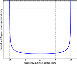
, the product of the average fade duration and the level crossing rate is a constant and is given by The Doppler power spectral density of a fading channel describes how much spectral broadening it causes.
For Rayleigh fading with a vertical receive antenna with equal sensitivity in all directions, this has been shown to be:[5] where
This spectrum is shown in the figure for a maximum Doppler shift of 10 Hz.
As described above, a Rayleigh fading channel itself can be modelled by generating the real and imaginary parts of a complex number according to independent normal Gaussian variables.
However, it is sometimes the case that it is simply the amplitude fluctuations that are of interest (such as in the figure shown above).
In both cases, the aim is to produce a signal that has the Doppler power spectrum given above and the equivalent autocorrelation properties.
In his book,[6] Jakes popularised a model for Rayleigh fading based on summing sinusoids.
A modified Jakes's model[8] chooses slightly different spacings for the scatterers and scales their waveforms using Walsh–Hadamard sequences to ensure zero cross-correlation.
The fast Walsh transform can be used to efficiently generate samples using this model.
Another way to generate a signal with the required Doppler power spectrum is to pass a white Gaussian noise signal through a Gaussian filter with a frequency response equal to the square-root of the Doppler spectrum required.
Although simpler than the models above, and non-deterministic, it presents some implementation questions related to needing high-order filters to approximate the irrational square-root function in the response and sampling the Gaussian waveform at an appropriate rate.
is the Cutoff frequency which should be selected with respect to maximum Doppler shift.