Romberg's method
In numerical analysis, Romberg's method[1] is used to estimate the definite integral
{\displaystyle \int _{a}^{b}f(x)\,dx}
by applying Richardson extrapolation[2] repeatedly on the trapezium rule or the rectangle rule (midpoint rule).
The estimates generate a triangular array.
Romberg's method is a Newton–Cotes formula – it evaluates the integrand at equally spaced points.
The integrand must have continuous derivatives, though fairly good results may be obtained if only a few derivatives exist.
If it is possible to evaluate the integrand at unequally spaced points, then other methods such as Gaussian quadrature and Clenshaw–Curtis quadrature are generally more accurate.
The method is named after Werner Romberg, who published the method in 1955.
{\textstyle h_{n}={\frac {(b-a)}{2^{n}}}}
, the method can be inductively defined by
{\displaystyle {\begin{aligned}R(0,0)&=h_{1}(f(a)+f(b))\\R(n,0)&={\tfrac {1}{2}}R(n-1,0)+h_{n}\sum _{k=1}^{2^{n-1}}f(a+(2k-1)h_{n})\\R(n,m)&=R(n,m-1)+{\tfrac {1}{4^{m}-1}}(R(n,m-1)-R(n-1,m-1))\\&={\frac {1}{4^{m}-1}}(4^{m}R(n,m-1)-R(n-1,m-1))\end{aligned}}}
In big O notation, the error for R(n, m) is:[3]
The zeroeth extrapolation, R(n, 0), is equivalent to the trapezoidal rule with 2n + 1 points; the first extrapolation, R(n, 1), is equivalent to Simpson's rule with 2n + 1 points.
The second extrapolation, R(n, 2), is equivalent to Boole's rule with 2n + 1 points.
The further extrapolations differ from Newton-Cotes formulas.
In particular further Romberg extrapolations expand on Boole's rule in very slight ways, modifying weights into ratios similar as in Boole's rule.
In contrast, further Newton-Cotes methods produce increasingly differing weights, eventually leading to large positive and negative weights.
This is indicative of how large degree interpolating polynomial Newton-Cotes methods fail to converge for many integrals, while Romberg integration is more stable.
By labelling our
, we can perform Richardson extrapolation with the error formula defined below:
Once we have obtained our
, we can label them as
When function evaluations are expensive, it may be preferable to replace the polynomial interpolation of Richardson with the rational interpolation proposed by Bulirsch & Stoer (1967).
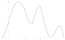
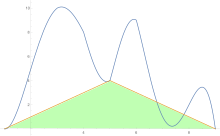
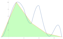
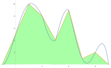
To estimate the area under a curve the trapezoid rule is applied first to one-piece, then two, then four, and so on.
After trapezoid rule estimates are obtained, Richardson extrapolation is applied.
As an example, the Gaussian function is integrated from 0 to 1, i.e. the error function erf(1) ≈ 0.842700792949715.
The triangular array is calculated row by row and calculation is terminated if the two last entries in the last row differ less than 10−8.
The result in the lower right corner of the triangular array is accurate to the digits shown.
It is remarkable that this result is derived from the less accurate approximations obtained by the trapezium rule in the first column of the triangular array.
Here is an example of a computer implementation of the Romberg method (in the C programming language): Here is an implementation of the Romberg method (in the Python programming language):