Shooting method
In numerical analysis, the shooting method is a method for solving a boundary value problem by reducing it to an initial value problem.
It involves finding solutions to the initial value problem for different initial conditions until one finds the solution that also satisfies the boundary conditions of the boundary value problem.
In layman's terms, one "shoots" out trajectories in different directions from one boundary until one finds the trajectory that "hits" the other boundary condition.
Suppose one wants to solve the boundary-value problem
The shooting method is the process of solving the initial value problem for many different values of
that satisfies the desired boundary conditions.
To systematically vary the shooting parameter
and find the root, one can employ standard root-finding algorithms like the bisection method or Newton's method.
and solutions to the boundary value problem are equivalent.
is a solution of the boundary value problem.
Conversely, if the boundary value problem has a solution
The term "shooting method" has its origin in artillery.
An analogy for the shooting method is to Between each shot, the direction of the cannon is adjusted based on the previous shot, so every shot hits closer than the previous one.
The trajectory that "hits" the desired boundary value is the solution to the boundary value problem — hence the name "shooting method".
The boundary value problem is linear if f has the form
In this case, the solution to the boundary value problem is usually given by:
is the solution to the initial value problem:
is the solution to the initial value problem:
See the proof for the precise condition under which this result holds.
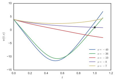
[1] A boundary value problem is given as follows by Stoer and Bulirsch[2] (Section 7.3.1).
Some trajectories of w(t;s) are shown in the Figure 1.
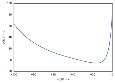
Stoer and Bulirsch[2] state that there are two solutions, which can be found by algebraic methods.
These correspond to the initial conditions w′(0) = −8 and w′(0) = −35.9 (approximately).The shooting method can also be used to solve eigenvalue problems.
Consider the time-independent Schrödinger equation for the quantum harmonic oscillator
In quantum mechanics, one seeks normalizable wavefunctions
and their corresponding energies subject to the boundary conditions
The problem can be solved analytically to find the energies
, but also serves as an excellent illustration of the shooting method.
To apply it, first note some general properties of the Schrödinger equation: To find the
, the shooting method is then to: The energy-guessing can be done with the bisection method, and the process can be terminated when the energy difference is sufficiently small.