Smith chart
[6][7][8][9][10] It was independently[11][4][12][5] proposed by Tōsaku Mizuhashi (水橋東作) in 1937,[13] and by Amiel R. Volpert [ru] (Амиэ́ль Р. Во́льперт)[14][4] and Phillip H. Smith in 1939.
[15][16] Starting with a rectangular diagram, Smith had developed a special polar coordinate chart by 1936, which, with the input of his colleagues Enoch B. Ferrell and James W. McRae, who were familiar with conformal mappings, was reworked into the final form in early 1937, which was eventually published in January 1939.
[18][19] The Smith chart can be used to simultaneously display multiple parameters including impedances, admittances, reflection coefficients,
scattering parameters, noise figure circles, constant gain contours and regions for unconditional stability.
[21]: 98–101 While the use of paper Smith charts for solving the complex mathematics involved in matching problems has been largely replaced by software based methods, the Smith chart is still a very useful method of showing[22] how RF parameters behave at one or more frequencies, an alternative to using tabular information.
If we are dealing only with impedances with non-negative resistive components, our interest is focused on the area inside the circle.
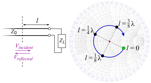
The wavelengths scale is used in distributed component problems and represents the distance measured along the transmission line connected between the generator or source and the load to the point under consideration.
Provided the frequencies are sufficiently close, the resulting Smith chart points may be joined by straight lines to create a locus.
A locus of points on a Smith chart covering a range of frequencies can be used to visually represent: The accuracy of the Smith chart is reduced for problems involving a large locus of impedances or admittances, although the scaling can be magnified for individual areas to accommodate these.
Therefore, This equation shows that, for a standing wave, the complex reflection coefficient and impedance repeats every half wavelength along the transmission line.
are the voltage across and the current entering the termination at the end of the transmission line respectively, then and By dividing these equations and substituting for both the voltage reflection coefficient and the normalised impedance of the termination represented by the lower case z, subscript T gives the result: Alternatively, in terms of the reflection coefficient These are the equations which are used to construct the Z Smith chart.
The Smith chart scaling is designed in such a way that reflection coefficient can be converted to normalised impedance or vice versa.
By substituting the expression for how reflection coefficient changes along an unmatched loss-free transmission line for the loss free case, into the equation for normalised impedance in terms of reflection coefficient and using Euler's formula yields the impedance-version transmission-line equation for the loss free case:[24] where
The path along the arc of the circle represents how the impedance changes whilst moving along the transmission line.
The magnitude of a complex number is the length of a straight line drawn from the origin to the point representing it.
If the termination is perfectly matched, the reflection coefficient will be zero, represented effectively by a circle of zero radius or in fact a point at the centre of the Smith chart.
In the complex reflection coefficient plane the Smith chart occupies a circle of unity radius centred at the origin.
Substituting these into the equation relating normalised impedance and complex reflection coefficient: gives the following result: This is the equation which describes how the complex reflection coefficient changes with the normalised impedance and may be used to construct both families of circles.
Again, if the termination is perfectly matched the reflection coefficient will be zero, represented by a 'circle' of zero radius or in fact a point at the centre of the Smith chart.
To graphically change this to the equivalent normalised admittance point, say Q1, a line is drawn with a ruler from P1 through the Smith chart centre to Q1, an equal radius in the opposite direction.
In general therefore, most RF engineers work in the plane where the circuit topography supports linear addition.
This occurs in microwave circuits and when high power requires large components in shortwave, FM and TV broadcasting.
For distributed components the effects on reflection coefficient and impedance of moving along the transmission line must be allowed for using the outer circumferential scale of the Smith chart which is calibrated in wavelengths.
The following example shows how a transmission line, terminated with an arbitrary load, may be matched at one frequency either with a series or parallel reactive component in each case connected at precise positions.
Reading from the Smith chart scaling, remembering that this is now a normalised admittance gives (In fact this value is not actually used).
The earliest point at which a shunt conjugate match could be introduced, moving towards the generator, would be at Q21, the same position as the previous P21, but this time representing a normalised admittance given by The distance along the transmission line is in this case which converts to 123 mm.
, then This gives the result A suitable inductive shunt matching would therefore be a 6.5 nH inductor in parallel with the line positioned at 123 mm from the load.
The following table shows the steps taken to work through the remaining components and transformations, returning eventually back to the centre of the Smith chart and a perfect 50 ohm match.
[26] The chart unifies the passive and active circuit design on little and big circles on the surface of a unit sphere, using a stereographic conformal map of the reflection coefficient's generalized plane.
[26] The 3D Smith chart has been further extended outside of the spherical surface, for plotting various scalar parameters, such as group delay, quality factors, or frequency orientation.