It occurs frequently in pure and applied mathematics, economics, quantitative finance, evolutionary biology, and physics.

The Wiener process plays an important role in both pure and applied mathematics.

In pure mathematics, the Wiener process gave rise to the study of continuous time martingales.

As such, it plays a vital role in stochastic calculus, diffusion processes and even potential theory.

In physics it is used to study Brownian motion and other types of diffusion via the Fokker–Planck and Langevin equations.

It also forms the basis for the rigorous path integral formulation of quantum mechanics (by the Feynman–Kac formula, a solution to the Schrödinger equation can be represented in terms of the Wiener process) and the study of eternal inflation in physical cosmology.

An alternative characterisation of the Wiener process is the so-called Lévy characterisation that says that the Wiener process is an almost surely continuous martingale with W0 = 0 and quadratic variation [Wt, Wt] = t (which means that Wt2 − t is also a martingale).

A third characterisation is that the Wiener process has a spectral representation as a sine series whose coefficients are independent N(0, 1) random variables.

Another characterisation of a Wiener process is the definite integral (from time zero to time t) of a zero mean, unit variance, delta correlated ("white") Gaussian process.

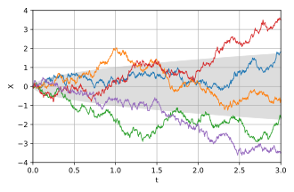
approaches a Wiener process, which explains the ubiquity of Brownian motion.

[6] The unconditional probability density function follows a normal distribution with mean = 0 and variance = t, at a fixed time t:

These results follow immediately from the definition that increments have a normal distribution, centered at zero.

These results follow from the definition that non-overlapping increments are independent, of which only the property that they are uncorrelated is used.

Wiener (1923) also gave a representation of a Brownian path in terms of a random Fourier series.

That is, a path (sample function) of the Wiener process has all these properties almost surely.

Consider that the local time can also be defined (as the density of the pushforward measure) for a smooth function.

In this sense, the continuity of the local time of the Wiener process is another manifestation of non-smoothness of the trajectory.

The information rate of the Wiener process with respect to the squared error distance, i.e. its quadratic rate-distortion function, is given by [9]

(in estimating the continuous-time Wiener process) follows the parametric representation [10]

is called a Wiener process with drift μ and infinitesimal variance σ2.

With no further conditioning, the process takes both positive and negative values on [0, 1] and is called Brownian bridge.

Conditioned also to stay positive on (0, 1), the process is called Brownian excursion.

[11] In both cases a rigorous treatment involves a limiting procedure, since the formula P(A|B) = P(A ∩ B)/P(B) does not apply when P(B) = 0.

The time of hitting a single point x > 0 by the Wiener process is a random variable with the Lévy distribution.

The family of these random variables (indexed by all positive numbers x) is a left-continuous modification of a Lévy process.

It arises in many applications and can be shown to have the distribution N(0, t3/3),[12] calculated using the fact that the covariance of the Wiener process is

The n-times-integrated Wiener process is a zero-mean normal variable with variance

Every continuous martingale (starting at the origin) is a time changed Wiener process.

Using this fact, the qualitative properties stated above for the Wiener process can be generalized to a wide class of continuous semimartingales.

The definition varies from authors, some define the Brownian sheet to have specifically a two-dimensional time parameter