Force between magnets
The forces of attraction and repulsion are a result of these interactions.
For homogeneous magnetization, the problem can be simplified in two different ways, using Stokes' theorem.
In both models, only two-dimensional distributions over the magnet's surface have to be considered, which is simpler than the original three-dimensional problem.
It is sometimes difficult to calculate the Ampèrian currents on the surface of a magnet.
In the physically correct Ampèrian loop model, magnetic dipole moments are due to infinitesimally small loops of current.
For a sufficiently small loop of current, I, and area, A, the magnetic dipole moment is:
As such, the SI unit of magnetic dipole moment is ampere meter2.
More precisely, to account for solenoids with many turns the unit of magnetic dipole moment is ampere–turn meter2.
In the magnetic pole model, the magnetic dipole moment is due to two equal and opposite magnetic charges that are separated by a distance, d. In this model, m is similar to the electric dipole moment p due to electrical charges:
The direction of the magnetic dipole moment points from the negative south pole to the positive north pole of this tiny magnet.
If like poles are facing each other, though, they are repulsed from the larger magnetic field.
The magnetic pole model predicts a correct mathematical form for this force and is easier to understand qualitatively.
The force obtained in the case of a current loop model is
where the gradient ∇ is the change of the quantity m · B per unit distance, and the direction is that of maximum increase of m · B.
To understand this equation, note that the dot product m · B = mB cos(θ), where m and B represent the magnitude of the m and B vectors and θ is the angle between them.
If m is in the same direction as B then the dot product is positive and the gradient points 'uphill' pulling the magnet into regions of higher B-field (more strictly larger m · B).
in the Ampèrian loop model, but this can be very cumbersome mathematically.
where The pole description is useful to practicing magneticians who design real-world magnets, but real magnets have a pole distribution more complex than a single north and south.
The mechanical force between two nearby magnetized surfaces can be calculated with the following equation.
The equation is valid only for cases in which the effect of fringing is negligible and the volume of the air gap is much smaller than that of the magnetized material, the force for each magnetized surface is:[2][3][4]
where: The derivation of this equation is analogous to the force between two nearby electrically charged surfaces,[5] which assumes that the field in between the plates is uniform.
Note that these formulations assume point-like magnetic-charge distributions instead of a uniform distribution over the end facets, which is a good approximation only at relatively great distances.
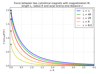
where With their magnetic dipole aligned, the force can be computed analytically using elliptic integrals.
, the results are erroneous as the force becomes large for close-to-zero distance.
Because of that, the strength of a permanent magnet can be expressed in the same terms as that of an electromagnet.
The strength of magnetism of an electromagnet that is a flat loop of wire through which a current flows, measured at a distance that is great compared to the size of the loop, is proportional to that current and is proportional to the surface area of that loop.
For purpose of expressing the strength of a permanent magnet in same terms as that of an electromagnet, a permanent magnet is thought of as if it contains small current-loops throughout its volume, and then the magnetic strength of that magnet is found to be proportional to the current of each loop (in amperes), and proportional to the surface of each loop (in square meters), and proportional to the density of current-loops in the material (in units per cubic meter), so the dimension of strength of magnetism of a permanent magnet is amperes times square meters per cubic meter, is amperes per meter.
This is very useful for computing magnetic force-field of a real magnet; It involves summing a large amount of small forces and you should not do that by hand, but let your computer do that for you; All that the computer program needs to know is the force between small magnets that are at great distance from each other.
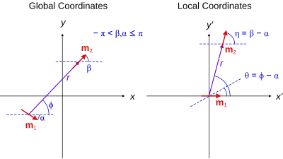
If the coordinate system is shifted to center it on m1 and rotated such that the x-axis points in the direction of m1 then the previous equation simplifies to[9]
This frame is called Local coordinates and is shown in the Figure on the right.


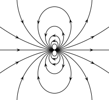
Bottom: , the force on aligned dipoles, such as iron particles.