Multimodal distribution
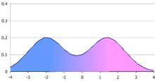
These appear as distinct peaks (local maxima) in the probability density function, as shown in Figures 1 and 2.
In time series the major mode is called the acrophase and the antimode the batiphase.
where a and b are constant and x and y are distributed as normal variables with a mean of 0 and a standard deviation of 1.
A t statistic generated from data set drawn from a Cauchy distribution is bimodal.
[3] Examples of variables with bimodal distributions include the time between eruptions of certain geysers, the color of galaxies, the size of worker weaver ants, the age of incidence of Hodgkin's lymphoma, the speed of inactivation of the drug isoniazid in US adults, the absolute magnitude of novae, and the circadian activity patterns of those crepuscular animals that are active both in morning and evening twilight.
In fishery science multimodal length distributions reflect the different year classes and can thus be used for age distribution- and growth estimates of the fish population.
When sampling mining galleries crossing either the host rock and the mineralized veins, the distribution of geochemical variables would be bimodal.
Bimodal distributions, despite their frequent occurrence in data sets, have only rarely been studied[citation needed].
It is not uncommon to encounter situations where an investigator believes that the data comes from a mixture of two normal distributions.
[15] Estimates of the parameters is simplified if the variances can be assumed to be equal (the homoscedastic case).
[19] Necessary and sufficient conditions for a mixture of normal distributions to be bimodal have been identified by Ray and Lindsay.
For example, in the distribution in Figure 1, the mean and median would be about zero, even though zero is not a typical value.
A value for A for each layer (Ai) is calculated and a weighted average for the distribution is determined.
It is related to a statistic proposed earlier by Pearson – the difference between the kurtosis and the square of the skewness (vide infra).
where Al and Ar are the amplitudes of the left and right peaks respectively and Pi is the logarithm taken to the base 2 of the proportion of the distribution in the ith interval.
It suffers from the usual problems of estimation and spectral leakage common to this form of statistic.
The authors suggested a cut off value of 0.1 for B to distinguish between a bimodal (B > 0.1)and unimodal (B < 0.1) distribution.
The φ-size is defined as minus one times the log of the data size taken to the base 2.
Otsu's method for finding a threshold for separation between two modes relies on minimizing the quantity
[36] A number of tests are available to determine if a data set is distributed in a bimodal (or multimodal) fashion.
An alternative method is to plot the log of the particle size against the cumulative frequency.
Equality holds only for the two point Bernoulli distribution or the sum of two different Dirac delta functions.
[41] Several tests of unimodality versus bimodality have been proposed: Haldane suggested one based on second central differences.
[48] Otsu's method is commonly employed in computer graphics to determine the optimal separation between two distributions.
Under smoothed densities may have an excessive number of modes whose count during bootstrapping is unstable.
[59] Additional tests are available for a number of special cases: A study of a mixture density of two normal distributions data found that separation into the two normal distributions was difficult unless the means were separated by 4–6 standard deviations.
[64] The mixtools package available for R can test for and estimate the parameters of a number of different distributions.
[66] Several other packages for R are available to fit mixture models; these include flexmix,[67] mcclust,[68] agrmt,[69] and mixdist.
[70] The statistical programming language SAS can also fit a variety of mixed distributions with the PROC FREQ procedure.
In Python, the package Scikit-learn contains a tool for mixture modeling[71] The CumFreqA [72] program for the fitting of composite probability distributions to a data set (X) can divide the set into two parts with a different distribution.