Unimodality
In mathematics, unimodality means possessing a unique mode.
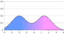
More generally, unimodality means there is only a single highest value, somehow defined, of some mathematical object.
If there is a single mode, the distribution function is called "unimodal".
[3] If the cdf is convex for x < m and concave for x > m, then the distribution is unimodal, m being the mode.
Criteria for unimodality can also be defined through the characteristic function of the distribution[3] or through its Laplace–Stieltjes transform.
[5] Another way to define a unimodal discrete distribution is by the occurrence of sign changes in the sequence of differences of the probabilities.
Thus, it is important to assess whether or not a given data set comes from a unimodal distribution.
[7] Gauss's inequality gives an upper bound on the probability that a value lies more than any given distance from its mode.
The Vysochanskiï–Petunin inequality refines this to even nearer values, provided that the distribution function is continuous and unimodal.
[9] Gauss also showed in 1823 that for a unimodal distribution[10] and where the median is ν, the mean is μ and ω is the root mean square deviation from the mode.
It can be shown for a unimodal distribution that the median ν and the mean μ lie within (3/5)1/2 ≈ 0.7746 standard deviations of each other.
In 2020, Bernard, Kazzi, and Vanduffel generalized the previous inequality by deriving the maximum distance between the symmetric quantile average
), which indeed motivates the common choice of the median as a robust estimator for the mean.
, which is the maximum distance between the median and the mean of a unimodal distribution.
A similar relation holds between the median and the mode θ: they lie within 31/2 ≈ 1.732 standard deviations of each other: It can also be shown that the mean and the mode lie within 31/2 of each other: Rohatgi and Szekely claimed that the skewness and kurtosis of a unimodal distribution are related by the inequality:[13] where κ is the kurtosis and γ is the skewness.
Klaassen, Mokveld, and van Es showed that this only applies in certain settings, such as the set of unimodal distributions where the mode and mean coincide.
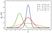
The definition of "unimodal" was extended to functions of real numbers as well.
A common definition is as follows: a function f(x) is a unimodal function if for some value m, it is monotonically increasing for x ≤ m and monotonically decreasing for x ≥ m. In that case, the maximum value of f(x) is f(m) and there are no other local maxima.
One way consists in using the definition of that property, but it turns out to be suitable for simple functions only.
A general method based on derivatives exists,[15] but it does not succeed for every function despite its simplicity.
A function f(x) is a weakly unimodal function if there exists a value m for which it is weakly monotonically increasing for x ≤ m and weakly monotonically decreasing for x ≥ m. In that case, the maximum value f(m) can be reached for a continuous range of values of x.
[16] For example, local unimodal sampling, a method for doing numerical optimization, is often demonstrated with such a function.
[19] A more general definition, applicable to a function f(X) of a vector variable X is that f is unimodal if there is a one-to-one differentiable mapping X = G(Z) such that f(G(Z)) is convex.
Usually one would want G(Z) to be continuously differentiable with nonsingular Jacobian matrix.