Chaos theory
[2] Chaos theory states that within the apparent randomness of chaotic complex systems, there are underlying patterns, interconnection, constant feedback loops, repetition, self-similarity, fractals and self-organization.
[8] This can happen even though these systems are deterministic, meaning that their future behavior follows a unique evolution[9] and is fully determined by their initial conditions, with no random elements involved.
[29] The flapping wing represents a small change in the initial condition of the system, which causes a chain of events that prevents the predictability of large-scale phenomena.
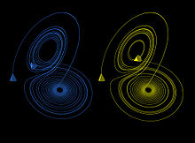
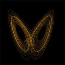
The Lorenz attractor is perhaps one of the best-known chaotic system diagrams, probably because it is not only one of the first, but it is also one of the most complex, and as such gives rise to a very interesting pattern that, with a little imagination, looks like the wings of a butterfly.
Other discrete dynamical systems have a repelling structure called a Julia set, which forms at the boundary between basins of attraction of fixed points.
[48] Since 1963, higher-dimensional Lorenz models have been developed in numerous studies[49][50][38][39] for examining the impact of an increased degree of nonlinearity, as well as its collective effect with heating and dissipations, on solution stability.
Examples include the coupled oscillation of Christiaan Huygens' pendulums, fireflies, neurons, the London Millennium Bridge resonance, and large arrays of Josephson junctions.
Later studies, also on the topic of nonlinear differential equations, were carried out by George David Birkhoff,[64] Andrey Nikolaevich Kolmogorov,[65][66][67] Mary Lucy Cartwright and John Edensor Littlewood,[68] and Stephen Smale.
As a graduate student in Chihiro Hayashi's laboratory at Kyoto University, Yoshisuke Ueda was experimenting with analog computers and noticed, on November 27, 1961, what he called "randomly transitional phenomena".
[14] Lorenz and his collaborator Ellen Fetter and Margaret Hamilton[77] were using a simple digital computer, a Royal McBee LGP-30, to run weather simulations.
In 1963, Benoit Mandelbrot, studying information theory, discovered that noise in many phenomena (including stock prices and telephone circuits) was patterned like a Cantor set, a set of points with infinite roughness and detail [79] Mandelbrot described both the "Noah effect" (in which sudden discontinuous changes can occur) and the "Joseph effect" (in which persistence of a value can occur for a while, yet suddenly change afterwards).
In 1979, Albert J. Libchaber, during a symposium organized in Aspen by Pierre Hohenberg, presented his experimental observation of the bifurcation cascade that leads to chaos and turbulence in Rayleigh–Bénard convection systems.
[86] In 1986, the New York Academy of Sciences co-organized with the National Institute of Mental Health and the Office of Naval Research the first important conference on chaos in biology and medicine.
In 1987, Per Bak, Chao Tang and Kurt Wiesenfeld published a paper in Physical Review Letters[88] describing for the first time self-organized criticality (SOC), considered one of the mechanisms by which complexity arises in nature.
Alongside largely lab-based approaches such as the Bak–Tang–Wiesenfeld sandpile, many other investigations have focused on large-scale natural or social systems that are known (or suspected) to display scale-invariant behavior.
[90] Initially the domain of a few, isolated individuals, chaos theory progressively emerged as a transdisciplinary and institutional discipline, mainly under the name of nonlinear systems analysis.
[94] Commencing with the 1960 conference in Japan, Lorenz embarked on a journey of developing diverse models aimed at uncovering the SDIC and chaotic features.
A recent review of Lorenz's model[95][96] progression spanning from 1960 to 2008 revealed his adeptness at employing varied physical systems to illustrate chaotic phenomena.
In 1972, Lorenz coined the term "butterfly effect" as a metaphor to discuss whether a small perturbation could eventually create a tornado with a three-dimensional, organized, and coherent structure.
While connected to the original butterfly effect based on sensitive dependence on initial conditions, its metaphorical variant carries distinct nuances.
Some areas benefiting from chaos theory today are geology, mathematics, biology, computer science, economics,[103][104][105] engineering,[106][107] finance,[108][109][110][111][112] meteorology, philosophy, anthropology,[16] physics,[113][114][115] politics,[116][117] population dynamics,[118] and robotics.
In fact, Orlando et al.[137] by the means of the so-called recurrence quantification correlation index were able detect hidden changes in time series.
Then, the same technique was employed to detect transitions from laminar (regular) to turbulent (chaotic) phases as well as differences between macroeconomic variables and highlight hidden features of economic dynamics.
[139] Due to the sensitive dependence of solutions on initial conditions (SDIC), also known as the butterfly effect, chaotic systems like the Lorenz 1963 model imply a finite predictability horizon.
Considering the nature of Lorenz's chaotic solutions, the committee led by Charney et al. in 1966 [140]extrapolated a doubling time of five days from a general circulation model, suggesting a predictability limit of two weeks.
This connection between the five-day doubling time and the two-week predictability limit was also recorded in a 1969 report by the Global Atmospheric Research Program (GARP).
In chemistry, predicting gas solubility is essential to manufacturing polymers, but models using particle swarm optimization (PSO) tend to converge to the wrong points.
They monitored the changes in between-heartbeat intervals for a single psychotherapy patient as she moved through periods of varying emotional intensity during a therapy session.
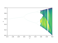
The authors were careful to test a large number of animals and to include many replications, and they designed their experiment so as to rule out the likelihood that changes in response patterns were caused by different starting places for r. Time series and first delay plots provide the best support for the claims made, showing a fairly clear march from periodicity to irregularity as the feeding times were increased.
[152] Modern organizations are increasingly seen as open complex adaptive systems with fundamental natural nonlinear structures, subject to internal and external forces that may contribute chaos.


![{\displaystyle [x,y]}](https://wikimedia.org/api/rest_v1/media/math/render/svg/1b7bd6292c6023626c6358bfd3943a031b27d663)