Decision tree

[citation needed] Another use of decision trees is as a descriptive means for calculating conditional probabilities.

Decision trees, influence diagrams, utility functions, and other decision analysis tools and methods are taught to undergraduate students in schools of business, health economics, and public health, and are examples of operations research or management science methods.

These tools are also used to predict decisions of householders in normal and emergency scenarios.

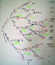
So used manually they can grow very big and are then often hard to draw fully by hand.

Traditionally, decision trees have been created manually – as the aside example shows – although increasingly, specialized software is employed.

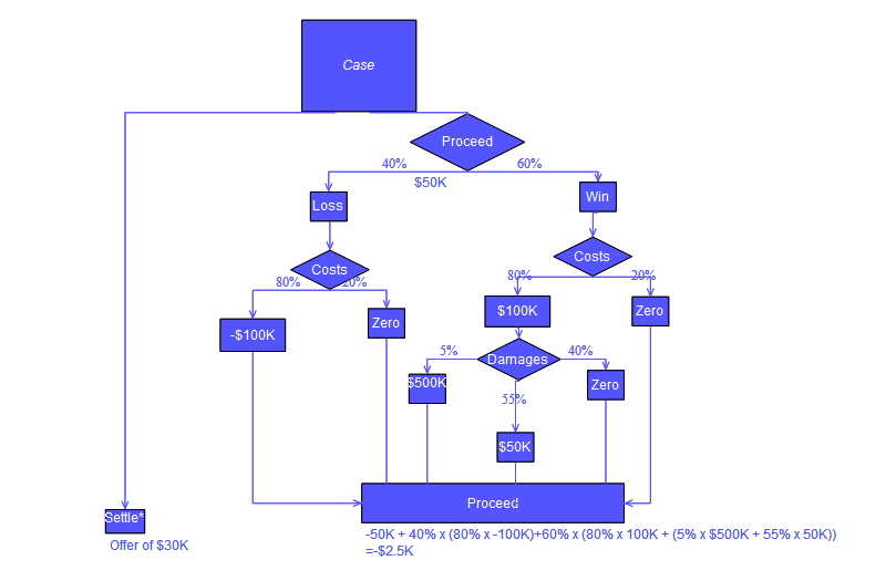
[6] Commonly a decision tree is drawn using flowchart symbols as it is easier for many to read and understand.

Analysis can take into account the decision maker's (e.g., the company's) preference or utility function, for example: The basic interpretation in this situation is that the company prefers B's risk and payoffs under realistic risk preference coefficients (greater than $400K—in that range of risk aversion, the company would need to model a third strategy, "Neither A nor B").

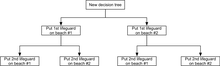
Another example, commonly used in operations research courses, is the distribution of lifeguards on beaches (a.k.a.

In this example, a decision tree can be drawn to illustrate the principles of diminishing returns on beach #1.

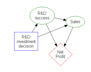
Much of the information in a decision tree can be represented more compactly as an influence diagram, focusing attention on the issues and relationships between events.

Decision trees can also be seen as generative models of induction rules from empirical data.

[8] Several algorithms to generate such optimal trees have been devised, such as ID3/4/5,[9] CLS, ASSISTANT, and CART.

[12] For example, if the classes in the data set are Cancer and Non-Cancer a leaf node would be considered pure when all the sample data in a leaf node is part of only one class, either cancer or non-cancer.

If the tree-building algorithm being used splits pure nodes, then a decrease in the overall accuracy of the tree classifier could be experienced.

We must be able to easily change and test the variables that could affect the accuracy and reliability of the decision tree-model.

The phi function is known as a measure of “goodness” of a candidate split at a node in the decision tree.

One decision tree will be built using the phi function to split the nodes and one decision tree will be built using the information gain function to split the nodes.

The formula states the information gain is a function of the entropy of a node of the decision tree minus the entropy of a candidate split at node t of a decision tree.

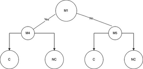
For example, if we use M1 to split the samples in the root node we get NC2 and C2 samples in group A and the rest of the samples NC4, NC3, NC1, C1 in group B. Disregarding the mutation chosen for the root node, proceed to place the next best features that have the highest values for information gain or the phi function in the left or right child nodes of the decision tree.

The leaves will represent the final classification decision the model has produced based on the mutations a sample either has or does not have.

Information gain confusion matrix: Phi function confusion matrix: The tree using information gain has the same results when using the phi function when calculating the accuracy.

The metrics that will be discussed below can help determine the next steps to be taken when optimizing the decision tree.

The ability to leverage the power of random forests can also help significantly improve the overall accuracy of the model being built.

There are many techniques, but the main objective is to test building your decision tree model in different ways to make sure it reaches the highest performance level possible.

All these measurements are derived from the number of true positives, false positives, True negatives, and false negatives obtained when running a set of samples through the decision tree classification model.

All these main metrics tell something different about the strengths and weaknesses of the classification model built based on your decision tree.

The confusion matrix shows us the decision tree model classifier built gave 11 true positives, 1 false positive, 45 false negatives, and 105 true negatives.

Once we have calculated the key metrics we can make some initial conclusions on the performance of the decision tree model built.

The accuracy value is good to start but we would like to get our models as accurate as possible while maintaining the overall performance.

[15] These are just a few examples on how to use these values and the meanings behind them to evaluate the decision tree model and improve upon the next iteration.