Gaussian function

for arbitrary real constants a, b and non-zero c. It is named after the mathematician Carl Friedrich Gauss.

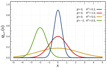
The graph of a Gaussian is a characteristic symmetric "bell curve" shape.

The parameter a is the height of the curve's peak, b is the position of the center of the peak, and c (the standard deviation, sometimes called the Gaussian RMS width) controls the width of the "bell".

Gaussian functions are often used to represent the probability density function of a normally distributed random variable with expected value μ = b and variance σ2 = c2.

Gaussian functions are widely used in statistics to describe the normal distributions, in signal processing to define Gaussian filters, in image processing where two-dimensional Gaussians are used for Gaussian blurs, and in mathematics to solve heat equations and diffusion equations and to define the Weierstrass transform.

They are also abundantly used in quantum chemistry to form basis sets.

The parameter c is related to the full width at half maximum (FWHM) of the peak according to

Alternatively, the parameter c can be interpreted by saying that the two inflection points of the function occur at x = b ± c. The full width at tenth of maximum (FWTM) for a Gaussian could be of interest and is

(the normalizing constant), and in this case the Gaussian is the probability density function of a normally distributed random variable with expected value μ = b and variance σ2 = c2:

The Fourier uncertainty principle becomes an equality if and only if (modulated) Gaussian functions are considered.

[2] Taking the Fourier transform (unitary, angular-frequency convention) of a Gaussian function with parameters a = 1, b = 0 and c yields another Gaussian function, with parameters

The fact that the Gaussian function is an eigenfunction of the continuous Fourier transform allows us to derive the following interesting[clarification needed] identity from the Poisson summation formula:

for some real constants a, b and c > 0 can be calculated by putting it into the form of a Gaussian integral.

In two dimensions, the power to which e is raised in the Gaussian function is any negative-definite quadratic form.

Here the coefficient A is the amplitude, x0, y0 is the center, and σx, σy are the x and y spreads of the blob.

In general, a two-dimensional elliptical Gaussian function is expressed as

For the general form of the equation the coefficient A is the height of the peak and (x0, y0) is the center of the blob.

(for negative, clockwise rotation, invert the signs in the b coefficient).

Example rotations of Gaussian blobs can be seen in the following examples: Using the following Octave code, one can easily see the effect of changing the parameters: Such functions are often used in image processing and in computational models of visual system function—see the articles on scale space and affine shape adaptation.

[5] This function may also be expressed in terms of the full width at half maximum (FWHM), represented by w:

A number of fields such as stellar photometry, Gaussian beam characterization, and emission/absorption line spectroscopy work with sampled Gaussian functions and need to accurately estimate the height, position, and width parameters of the function.

The most common method for estimating the Gaussian parameters is to take the logarithm of the data and fit a parabola to the resulting data set.

[7][8] While this provides a simple curve fitting procedure, the resulting algorithm may be biased by excessively weighting small data values, which can produce large errors in the profile estimate.

One can partially compensate for this problem through weighted least squares estimation, reducing the weight of small data values, but this too can be biased by allowing the tail of the Gaussian to dominate the fit.

[8] It is also possible to perform non-linear regression directly on the data, without involving the logarithmic data transformation; for more options, see probability distribution fitting.

[9][10] When these assumptions are satisfied, the following covariance matrix K applies for the 1D profile parameters

Thus, the individual variances for the parameters are, in the Gaussian noise case,

where the individual parameter variances are given by the diagonal elements of the covariance matrix.

However, this discrete function does not have the discrete analogs of the properties of the continuous function, and can lead to undesired effects, as described in the article scale space implementation.

denotes the modified Bessel functions of integer order.