Generalized coordinates

In analytical mechanics, generalized coordinates are a set of parameters used to represent the state of a system in a configuration space.

These parameters must uniquely define the configuration of the system relative to a reference state.

However, it can also occur that a useful set of generalized coordinates may be dependent, which means that they are related by one or more constraint equations.

If it is possible to find from the constraints as many independent variables as there are degrees of freedom, these can be used as generalized coordinates.

In the case the constraints on the particles are time-independent, then all partial derivatives with respect to time are zero, and the kinetic energy is a homogeneous function of degree 2 in the generalized velocities.

Still for the time-independent case, this expression is equivalent to taking the line element squared of the trajectory for particle k, and dividing by the square differential in time, dt2, to obtain the velocity squared of particle k. Thus for time-independent constraints it is sufficient to know the line element to quickly obtain the kinetic energy of particles and hence the Lagrangian.

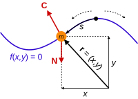
In 2D polar coordinates (r, θ), in 3D cylindrical coordinates (r, θ, z), in 3D spherical coordinates (r, θ, φ), The generalized momentum "canonically conjugate to" the coordinate qi is defined by If the Lagrangian L does not depend on some coordinate qi, then it follows from the Euler–Lagrange equations that the corresponding generalized momentum will be a conserved quantity, because the time derivative is zero implying the momentum is a constant of the motion; For a bead sliding on a frictionless wire subject only to gravity in 2d space, the constraint on the bead can be stated in the form f (r) = 0, where the position of the bead can be written r = (x(s), y(s)), in which s is a parameter, the arc length s along the curve from some point on the wire.

Notice time appears implicitly via the coordinates and explicitly in the constraint equations.

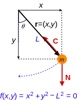
[12][13] A simple pendulum consists of a mass M hanging from a pivot point so that it is constrained to move on a circle of radius L. The position of the mass is defined by the coordinate vector r = (x, y) measured in the plane of the circle such that y is in the vertical direction.

The virtual work of gravity on the mass m as it follows the trajectory r is given by The variation δr can be computed in terms of the coordinates x and y, or in terms of the parameter θ, Thus, the virtual work is given by Notice that the coefficient of δy is the y-component of the applied force.

In the same way, the coefficient of δθ is known as the generalized force along generalized coordinate θ, given by To complete the analysis consider the kinetic energy T of the mass, using the velocity, so, D'Alembert's form of the principle of virtual work for the pendulum in terms of the coordinates x and y are given by, This yields the three equations in the three unknowns, x, y and λ.

Now introduce the generalized coordinates θi (i = 1, 2) that define the angular position of each mass of the double pendulum from the vertical direction.

Therefore, the virtual work of gravity on the two masses as they follow the trajectories ri (i = 1, 2) is given by The variations δri (i = 1, 2) can be computed to be Thus, the virtual work is given by and the generalized forces are Compute the kinetic energy of this system to be Euler–Lagrange equation yield two equations in the unknown generalized coordinates θi (i = 1, 2) given by[14] and The use of the generalized coordinates θi (i = 1, 2) provides an alternative to the Cartesian formulation of the dynamics of the double pendulum.

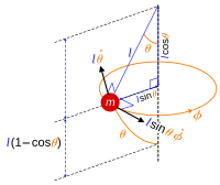
A logical choice of generalized coordinates to describe the motion are the angles (θ, φ).