Contrast (vision)
[1] The human visual system is more sensitive to contrast than to absolute luminance; thus, we can perceive the world similarly despite significant changes in illumination throughout the day or across different locations.
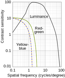
Campbell and Robson (1968) showed that the human contrast sensitivity function shows a typical band-pass filter shape peaking at around 4 cycles per degree (cpd or cyc/deg), with sensitivity dropping off either side of the peak.
[3] This can be observed by changing one's viewing distance from a "sweep grating" (shown below) showing many bars of a sinusoidal grating that go from high to low contrast along the bars, and go from narrow (high spatial frequency) to wide (low spatial frequency) bars across the width of the grating.
The high-frequency cut-off represents the optical limitations of the visual system's ability to resolve detail and is typically about 60 cpd.
The low frequency drop-off is due to lateral inhibition within the retinal ganglion cells.
[4] A typical retinal ganglion cell's receptive field comprises a central region in which light either excites or inhibits the cell, and a surround region in which light has the opposite effects.
Since white minus blue is red and green, this mixes to become yellow.
Russian scientist N. P. Travnikova [d] laments, "Such a multiplicity of notions of contrast is extremely inconvenient.
It complicates the solution of many applied problems and makes it difficult to compare the results published by different authors.
In many cases, the definitions of contrast represent a ratio of the type The rationale behind this is that a small difference is negligible if the average luminance is high, while the same small difference matters if the average luminance is low (see Weber–Fechner law).
Weber contrast is commonly used in cases where small features are present on a large uniform background, i.e., where the average luminance is approximately equal to the background luminance.Michelson contrast[8] (also known as the visibility) is commonly used for patterns where both bright and dark features are equivalent and take up similar fractions of the area (e.g. sine-wave gratings).
Contrast sensitivity is a measure of the ability to discern different luminances in a static image.
Factors such as cataracts and diabetic retinopathy also reduce contrast sensitivity.
[12] In the sweep grating figure below, at an ordinary viewing distance, the bars in the middle appear to be the longest due to their optimal spatial frequency.
[13] For example, some individuals with glaucoma may achieve 20/20 vision on acuity exams, yet struggle with activities of daily living, such as driving at night.
As mentioned above, contrast sensitivity describes the ability of the visual system to distinguish bright and dim components of a static image.
Visual acuity can be defined as the angle with which one can resolve two points as being separate since the image is shown with 100% contrast and is projected onto the fovea of the retina.
[14] Thus, when an optometrist or ophthalmologist assesses a patient's visual acuity using a Snellen chart or some other acuity chart, the target image is displayed at high contrast, e.g., black letters of decreasing size on a white background.
Most charts in an ophthalmologist's or optometrist's office will show images of varying contrast and spatial frequency.
Parallel bars of varying width and contrast, known as sine-wave gratings, are sequentially viewed by the patient.
[17] Recent studies have demonstrated that intermediate-frequency sinusoidal patterns are optimally-detected by the retina due to the center-surround arrangement of neuronal receptive fields.
[18] In an intermediate spatial frequency, the peak (brighter bars) of the pattern is detected by the center of the receptive field, while the troughs (darker bars) are detected by the inhibitory periphery of the receptive field.
[19] Other environmental,[20] physiological, and anatomical factors influence the neuronal transmission of sinusoidal patterns, including adaptation.
[21] Decreased contrast sensitivity arises from multiple etiologies, including retinal disorders such as age-related macular degeneration (ARMD), amblyopia, lens abnormalities, such as cataract, and by higher-order neural dysfunction, including stroke and Alzheimer's disease.
A large-scale study of luminance contrast thresholds was done in the 1940s by Blackwell,[23] using a forced-choice procedure.
The resulting data have been used extensively in areas such as lighting engineering and road safety.
A mathematical formula for the resulting threshold curve was proposed by Hecht,[27] with separate branches for scotopic and photopic vision.
Crumey[24] showed that Hecht's formula fitted the data very poorly at low light levels, so was not really suitable for modelling stellar visibility.
Crumey instead constructed a more accurate and general model applicable to both the Blackwell and Knoll et al data.
Crumey used it to model astronomical visibility for targets of arbitrary size, and to study the effects of light pollution.