Kernel density estimation

In statistics, kernel density estimation (KDE) is the application of kernel smoothing for probability density estimation, i.e., a non-parametric method to estimate the probability density function of a random variable based on kernels as weights.

In some fields such as signal processing and econometrics it is also termed the Parzen–Rosenblatt window method, after Emanuel Parzen and Murray Rosenblatt, who are usually credited with independently creating it in its current form.

[1][2] One of the famous applications of kernel density estimation is in estimating the class-conditional marginal densities of data when using a naive Bayes classifier, which can improve its prediction accuracy.

Intuitively one wants to choose h as small as the data will allow; however, there is always a trade-off between the bias of the estimator and its variance.

A range of kernel functions are commonly used: uniform, triangular, biweight, triweight, Epanechnikov (parabolic), normal, and others.

Similar methods are used to construct discrete Laplace operators on point clouds for manifold learning (e.g. diffusion map).

The diagram below based on these 6 data points illustrates this relationship: For the histogram, first, the horizontal axis is divided into sub-intervals or bins which cover the range of the data: In this case, six bins each of width 2.

Whenever a data point falls inside this interval, a box of height 1/12 is placed there.

If more than one data point falls inside the same bin, the boxes are stacked on top of each other.

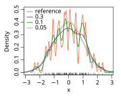
[7] The bandwidth of the kernel is a free parameter which exhibits a strong influence on the resulting estimate.

To illustrate its effect, we take a simulated random sample from the standard normal distribution (plotted at the blue spikes in the rug plot on the horizontal axis).

In comparison, the red curve is undersmoothed since it contains too many spurious data artifacts arising from using a bandwidth h = 0.05, which is too small.

The green curve is oversmoothed since using the bandwidth h = 2 obscures much of the underlying structure.

(no smoothing), where the estimate is a sum of n delta functions centered at the coordinates of analyzed samples.

the estimate retains the shape of the used kernel, centered on the mean of the samples (completely smooth).

The most common optimality criterion used to select this parameter is the expected L2 risk function, also termed the mean integrated squared error: Under weak assumptions on ƒ and K, (ƒ is the, generally unknown, real density function),[1][2] where o is the little o notation, and n the sample size (as above).

To overcome that difficulty, a variety of automatic, data-based methods have been developed to select the bandwidth.

Several review studies have been undertaken to compare their efficacies,[8][9][10][11][12][13][14] with the general consensus that the plug-in selectors[6][15][16] and cross validation selectors[17][18][19] are the most useful over a wide range of data sets.

Bandwidth selection for kernel density estimation of heavy-tailed distributions is relatively difficult.

[21] If Gaussian basis functions are used to approximate univariate data, and the underlying density being estimated is Gaussian, the optimal choice for h (that is, the bandwidth that minimises the mean integrated squared error) is:[22] An

[22] While this rule of thumb is easy to compute, it should be used with caution as it can yield widely inaccurate estimates when the density is not close to being normal.

For example, when estimating the bimodal Gaussian mixture model from a sample of 200 points, the figure on the right shows the true density and two kernel density estimates — one using the rule-of-thumb bandwidth, and the other using a solve-the-equation bandwidth.

[6][16] The estimate based on the rule-of-thumb bandwidth is significantly oversmoothed.

One difficulty with applying this inversion formula is that it leads to a diverging integral, since the estimate

is multiplied by a damping function ψh(t) = ψ(ht), which is equal to 1 at the origin and then falls to 0 at infinity.

The “bandwidth parameter” h controls how fast we try to dampen the function

In particular when h is small, then ψh(t) will be approximately one for a large range of t’s, which means that

is the collection of points for which the density function is locally maximized.

Note that one can use the mean shift algorithm[25][26][27] to compute the estimator

A non-exhaustive list of software implementations of kernel density estimators includes: