AD–AS model
From around 2000 the modified version of a dynamic AD–AS model, incorporating contemporary monetary policy strategies focusing on inflation targeting and using the interest rate as a primary policy instrument, was developed, gradually superseding the traditional static model version in university-level economics textbooks.
At the same time, the latter is much simpler and consequently more easily accessible for students, making it a widespread tool for teaching purposes.
[1][2] In particular, two intermediate textbooks appearing in 1978 and later to be widely used, one by Rudi Dornbusch and Stanley Fischer, and one by Robert J. Gordon, together with William Hoban Branson's texbook from its second edition in 1979, all presented an AD–AS model.
[2][3][4] Because of that, the original AD–AS model has increasingly been supplanted in textbooks by a dynamic version which directly analyzes equilibria in output and inflation levels, showing these variables along the axes of the diagram.
[3][4][5] In some textbooks, the dynamic AD–AS version is referred to as the "three-equation New Keynesian model",[6] the three equations being an IS relation, often augmented with a term that allows for expectations influencing demand, a monetary policy (interest) rule and a short-run Phillips curve.
[7] Olivier Blanchard in his widely-used[8] intermediate-level textbook uses the term IS–LM–PC model (PC standing for Phillips curve) for the same basic construction.
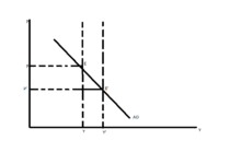
[10] Movements of the two curves can be used to predict the effects that various exogenous events will have on two variables: real GDP and the price level.
[5]: 266 Under the premise that the price level is flexible in the long run, but sticky or even completely fixed under shorter time horizons, it is usual to distinguish between a long-run and a short-run aggregate supply curve.
[5]: 268 The equation for the aggregate supply curve in general terms may be written as where W is the nominal wage rate (exogenous due to stickiness in the short run), Pe is the anticipated (expected) price level, and Z2 is a vector of exogenous variables that can affect the position of the labor demand curve.
One possible justification for this is that when there is unemployment, firms can readily obtain as much labour as they want at that current wage, and production can increase without any additional costs (e.g. machines are idle which can simply be turned on).
The long-run aggregate supply curve refers not to a time frame in which the capital stock is free to be set optimally (as would be the terminology in the micro-economic theory of the firm), but rather to a time frame in which wages are free to adjust in order to equilibrate the labor market and in which price anticipations are accurate.
[5]: 411 Changes in the level of potential Y also shifts the AD curve, so that this type of shocks has an effect on both the supply and the demand side of the model.