Signal-flow graph

Wai-Kai Chen wrote: "The concept of a signal-flow graph was originally worked out by Shannon [1942][1] in dealing with analog computers.

[5] He showed how to use the signal-flow graph technique to solve some difficult electronic problems in a relatively simple manner.

Three years later, Mason [1956] rediscovered the rules and proved them by considering the value of a determinant and how it changes as variables are added to the graph.

"A flow graph, as defined originally by Mason, implies a set of functional relations, linear or not.

Frequently these functions are simply multiplicative factors (often called transmittances or gains), for example, fij(xj)=cijxj, where c is a scalar, but possibly a function of some parameter like the Laplace transform variable s. Signal-flow graphs are very often used with Laplace-transformed signals, because then they represent systems of Linear differential equations.

One system will give different graphs according to the order in which the equations are used to define the variable written on the left-hand side.

These incoming branches convey the contributions of the other nodes, expressed as the connected node value multiplied by the weight of the connecting branch, usually a real number or function of some parameter (for example a Laplace transform variable s).

For linear active networks, Choma writes:[14] "By a 'signal flow representation' [or 'graph', as it is commonly referred to] we mean a diagram that, by displaying the algebraic relationships among relevant branch variables of network, paints an unambiguous picture of the way an applied input signal ‘flows’ from input-to-output ...

A motivation for a SFG analysis is described by Chen:[15] A linear signal flow graph is related to a system of linear equations[16] of the following form: The figure to the right depicts various elements and constructs of a signal flow graph (SFG).

[23] The rules presented below may be applied over and over until the signal flow graph is reduced to its "minimal residual form".

Further reduction can require loop elimination or the use of a "reduction formula" with the goal to directly connect sink nodes representing the dependent variables to the source nodes representing the independent variables.

This method is close to the familiar process of successive eliminations of undesired variables in a system of equations.

Replace looping edges by adjusting the gains on the incoming edges.The graph on the left has a looping edge at node N, with a gain of g. On the right, the looping edge has been eliminated, and all inflowing edges have their gain divided by (1-g).The equations corresponding to the reduction between N and all its input signals are: The above procedure for building the SFG from an acausal system of equations and for solving the SFG's gains have been implemented[31] as an add-on to MATHLAB 68,[32] an on-line system providing machine aid for the mechanical symbolic processes encountered in analysis.

Every equation is treated this way, and then each incident branch is joined to its respective emanating node.

When expressed using the general coefficients {cin}, the environment of each node is then just like all the rest apart from a permutation of indices.

In general, there are N-1 paths from yj to variable xk so the computational effort to calculated Gkj is proportional to N-1.

[38] According to Barker et al.:[39] In the figure, a simple block diagram for a feedback system is shown with two possible interpretations as a signal-flow graph.

G(s) and H(s) are transfer functions, with H(s) serving to feed back a modified version of the output to the input, B(s).

The term "cause and effect" was applied by Mason to SFGs:[2] and has been repeated by many later authors:[40] However, Mason's paper is concerned to show in great detail how a set of equations is connected to an SFG, an emphasis unrelated to intuitive notions of "cause and effect".

The essential connection of the SFG is to its own set of equations, as described, for example, by Ogata:[41] There is no reference to "cause and effect" here, and as said by Barutsky:[42] The term "cause and effect" may be misinterpreted as it applies to the SFG, and taken incorrectly to suggest a system view of causality,[43] rather than a computationally based meaning.

[46] Signal-flow graphs can be used for analysis, that is for understanding a model of an existing system, or for synthesis, that is for determining the properties of a design alternative.

Signal-flow graphs have been used in Design Space Exploration (DSE), as an intermediate representation towards a physical implementation.

In contrast with the typical analysis workflow, where a system of interest is first modeled with the physical equations of its components, the specification for synthesizing a design could be a desired transfer function.

During World War II, while investigating the functional operation of an analog computer, Claude Shannon developed his formula.

Because of wartime restrictions, Shannon's work was not published at that time, and, in 1952, Mason rediscovered the same formula.

[51] For a consistent set of linear unilateral relations, the Shannon-Happ formula expresses the solution using direct substitution (non-iterative).

[53] A possible SFG for the asymptotic gain model for a negative feedback amplifier is shown in Figure 3, and leads to the equation for the gain of this amplifier as The interpretation of the parameters is as follows: T = return ratio, G∞ = direct amplifier gain, G0 = feedforward (indicating the possible bilateral nature of the feedback, possibly deliberate as in the case of feedforward compensation).

Figure 4 shows another SFG for the asymptotic gain model that can be easier to interpret in terms of a circuit.

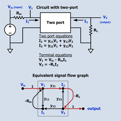
The two-port equations impose a set of linear constraints between its port voltages and currents.

Compared to the schematic, the SFG is awkward but it does have the advantage that the input to output gain can be written down by inspection using Mason's rule.