Mathematical visualization
In contrast, today it most frequently consists of using computers to make static two- or three-dimensional drawings, animations, or interactive programs.
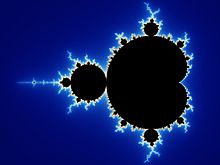
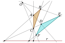
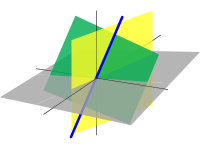
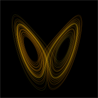
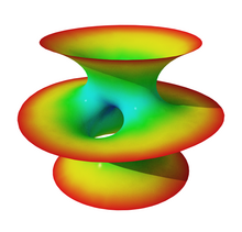
Notable examples include plane curves, space curves, polyhedra, ordinary differential equations, partial differential equations (particularly numerical solutions, as in fluid dynamics or minimal surfaces such as soap films), conformal maps, fractals, and chaos.
Extending to 3 dimensions the physically impossible Riemann surfaces used to classify all closed orientable 2-manifolds, Heegaard's 1898 thesis "looked at" similar structures for functions of two complex variables, taking an imaginary 4-dimensional surface in Euclidean 6-space (corresponding to the function f=x^2-y^3) and projecting it stereographically (with multiplicities) onto the 3-sphere.
In the 1920s Alexander and Briggs used this technique to compute the homology of cyclic branched covers of knots with 8 or fewer crossings, successfully distinguishing them all from each other (and the unknot).
By 1932 Reidemeister extended this to 9 crossings, relying on linking numbers between branch curves of non-cyclic knot covers.