Nonlinear system

Collective intelligence Collective action Self-organized criticality Herd mentality Phase transition Agent-based modelling Synchronization Ant colony optimization Particle swarm optimization Swarm behaviour Social network analysis Small-world networks Centrality Motifs Graph theory Scaling Robustness Systems biology Dynamic networks Evolutionary computation Genetic algorithms Genetic programming Artificial life Machine learning Evolutionary developmental biology Artificial intelligence Evolutionary robotics Reaction–diffusion systems Partial differential equations Dissipative structures Percolation Cellular automata Spatial ecology Self-replication Conversation theory Entropy Feedback Goal-oriented Homeostasis Information theory Operationalization Second-order cybernetics Self-reference System dynamics Systems science Systems thinking Sensemaking Variety Ordinary differential equations Phase space Attractors Population dynamics Chaos Multistability Bifurcation Rational choice theory Bounded rationality In mathematics and science, a nonlinear system (or a non-linear system) is a system in which the change of the output is not proportional to the change of the input.

[8] Nonlinear dynamical systems, describing changes in variables over time, may appear chaotic, unpredictable, or counterintuitive, contrasting with much simpler linear systems.

Typically, the behavior of a nonlinear system is described in mathematics by a nonlinear system of equations, which is a set of simultaneous equations in which the unknowns (or the unknown functions in the case of differential equations) appear as variables of a polynomial of degree higher than one or in the argument of a function which is not a polynomial of degree one.

In other words, in a nonlinear system of equations, the equation(s) to be solved cannot be written as a linear combination of the unknown variables or functions that appear in them.

Systems can be defined as nonlinear, regardless of whether known linear functions appear in the equations.

In particular, a differential equation is linear if it is linear in terms of the unknown function and its derivatives, even if nonlinear in terms of the other variables appearing in it.

As nonlinear dynamical equations are difficult to solve, nonlinear systems are commonly approximated by linear equations (linearization).

This works well up to some accuracy and some range for the input values, but some interesting phenomena such as solitons, chaos,[9] and singularities are hidden by linearization.

It follows that some aspects of the dynamic behavior of a nonlinear system can appear to be counterintuitive, unpredictable or even chaotic.

For example, some aspects of the weather are seen to be chaotic, where simple changes in one part of the system produce complex effects throughout.

This nonlinearity is one of the reasons why accurate long-term forecasts are impossible with current technology.

This term is disputed by others: Using a term like nonlinear science is like referring to the bulk of zoology as the study of non-elephant animals.In mathematics, a linear map (or linear function)

The conditions of additivity and homogeneity are often combined in the superposition principle An equation written as is called linear if

can literally be any mapping, including integration or differentiation with associated constraints (such as boundary values).

Solving systems of polynomial equations, that is finding the common zeros of a set of several polynomials in several variables is a difficult problem for which elaborated algorithms have been designed, such as Gröbner base algorithms.

[11] For the general case of system of equations formed by equating to zero several differentiable functions, the main method is Newton's method and its variants.

[12] These approaches can be used to study a wide class of complex nonlinear behaviors in the time, frequency, and spatio-temporal domains.

A good example of this is one-dimensional heat transport with Dirichlet boundary conditions, the solution of which can be written as a time-dependent linear combination of sinusoids of differing frequencies; this makes solutions very flexible.

Second and higher order ordinary differential equations (more generally, systems of nonlinear equations) rarely yield closed-form solutions, though implicit solutions and solutions involving nonelementary integrals are encountered.

Common methods for the qualitative analysis of nonlinear ordinary differential equations include: The most common basic approach to studying nonlinear partial differential equations is to change the variables (or otherwise transform the problem) so that the resulting problem is simpler (possibly linear).

Another common (though less mathematical) tactic, often exploited in fluid and heat mechanics, is to use scale analysis to simplify a general, natural equation in a certain specific boundary value problem.

For example, the (very) nonlinear Navier-Stokes equations can be simplified into one linear partial differential equation in the case of transient, laminar, one dimensional flow in a circular pipe; the scale analysis provides conditions under which the flow is laminar and one dimensional and also yields the simplified equation.

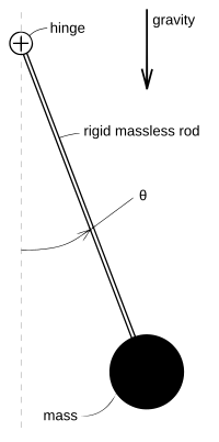
A classic, extensively studied nonlinear problem is the dynamics of a frictionless pendulum under the influence of gravity.

Using Lagrangian mechanics, it may be shown[14] that the motion of a pendulum can be described by the dimensionless nonlinear equation where gravity points "downwards" and

is the angle the pendulum forms with its rest position, as shown in the figure at right.

Another way to approach the problem is to linearize any nonlinearity (the sine function term in this case) at the various points of interest through Taylor expansions.

The solution to this problem involves hyperbolic sinusoids, and note that unlike the small angle approximation, this approximation is unstable, meaning that

This corresponds to the difficulty of balancing a pendulum upright, it is literally an unstable state.

A very useful qualitative picture of the pendulum's dynamics may be obtained by piecing together such linearizations, as seen in the figure at right.

Other techniques may be used to find (exact) phase portraits and approximate periods.