Phase space
For mechanical systems, the phase space usually consists of all possible values of the position and momentum parameters.
[clarification needed] The concept of phase space was developed in the late 19th century by Ludwig Boltzmann, Henri Poincaré, and Josiah Willard Gibbs.
The phase-space trajectory represents the set of states compatible with starting from one particular initial condition, located in the full phase space that represents the set of states compatible with starting from any initial condition.
Phase spaces are easier to use when analyzing the behavior of mechanical systems restricted to motion around and along various axes of rotation or translation – e.g. in robotics, like analyzing the range of motion of a robotic arm or determining the optimal path to achieve a particular position/momentum result.
Because of this, it is possible to calculate the state of the system at any given time in the future or the past, through integration of Hamilton's or Lagrange's equations of motion.
One degree of freedom occurs when one has an autonomous ordinary differential equation in a single variable,
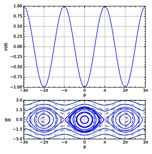
In this case, a sketch of the phase portrait may give qualitative information about the dynamics of the system, such as the limit cycle of the Van der Pol oscillator shown in the diagram.
This reveals information such as whether an attractor, a repellor or limit cycle is present for the chosen parameter value.
The concept of topological equivalence is important in classifying the behaviour of systems by specifying when two different phase portraits represent the same qualitative dynamic behavior.
But they may alternatively retain their classical interpretation, provided functions of them compose in novel algebraic ways (through Groenewold's 1946 star product).
Every quantum mechanical observable corresponds to a unique function or distribution on phase space, and conversely, as specified by Hermann Weyl (1927) and supplemented by John von Neumann (1931); Eugene Wigner (1932); and, in a grand synthesis, by H. J. Groenewold (1946).
Expectation values in phase-space quantization are obtained isomorphically to tracing operator observables with the density matrix in Hilbert space: they are obtained by phase-space integrals of observables, with the Wigner quasi-probability distribution effectively serving as a measure.
)[citation needed] Classical expressions, observables, and operations (such as Poisson brackets) are modified by ħ-dependent quantum corrections, as the conventional commutative multiplication applying in classical mechanics is generalized to the noncommutative star-multiplication characterizing quantum mechanics and underlying its uncertainty principle.
In this sense, as long as the particles are distinguishable, a point in phase space is said to be a microstate of the system.
N is typically on the order of the Avogadro number, thus describing the system at a microscopic level is often impractical.