Ordinary least squares

Under these conditions, the method of OLS provides minimum-variance mean-unbiased estimation when the errors have finite variances.

This formulation highlights the point that estimation can be carried out if, and only if, there is no perfect multicollinearity between the explanatory variables (which would cause the Gram matrix to have no inverse).

In order for R2 to be meaningful, the matrix X of data on regressors must contain a column vector of ones to represent the constant whose coefficient is the regression intercept.

If the data matrix X contains only two variables, a constant and a scalar regressor xi, then this is called the "simple regression model".

This case is often considered in the beginner statistics classes, as it provides much simpler formulas even suitable for manual calculation.

For mathematicians, OLS is an approximate solution to an overdetermined system of linear equations Xβ ≈ y, where β is the unknown.

Thus, the residual vector y − Xβ will have the smallest length when y is projected orthogonally onto the linear subspace spanned by the columns of X.

[16][proof] This normality assumption has historical importance, as it provided the basis for the early work in linear regression analysis by Yule and Pearson.

[citation needed] From the properties of MLE, we can infer that the OLS estimator is asymptotically efficient (in the sense of attaining the Cramér–Rao bound for variance) if the normality assumption is satisfied.

Since xi is a p-vector, the number of moment conditions is equal to the dimension of the parameter vector β, and thus the system is exactly identified.

Note that the original strict exogeneity assumption E[εi | xi] = 0 implies a far richer set of moment conditions than stated above.

There are several different frameworks in which the linear regression model can be cast in order to make the OLS technique applicable.

The choice of the applicable framework depends mostly on the nature of data in hand, and on the inference task which has to be performed.

The classical model focuses on the "finite sample" estimation and inference, meaning that the number of observations n is fixed.

In some applications, especially with cross-sectional data, an additional assumption is imposed — that all observations are independent and identically distributed.

This means that all observations are taken from a random sample which makes all the assumptions listed earlier simpler and easier to interpret.

Also this framework allows one to state asymptotic results (as the sample size n → ∞), which are understood as a theoretical possibility of fetching new independent observations from the data generating process.

and s2 are unbiased, meaning that their expected values coincide with the true values of the parameters:[24][proof] If the strict exogeneity does not hold (as is the case with many time series models, where exogeneity is assumed only with respect to the past shocks but not the future ones), then these estimators will be biased in finite samples.

[17] Note that unlike the Gauss–Markov theorem, this result establishes optimality among both linear and non-linear estimators, but only in the case of normally distributed error terms.

[32] Usually the observations with high leverage ought to be scrutinized more carefully, in case they are erroneous, or outliers, or in some other way atypical of the rest of the dataset.

However it may happen that adding the restriction A makes β identifiable, in which case one would like to find the formula for the estimator.

Nevertheless, we can apply the central limit theorem to derive their asymptotic properties as sample size n goes to infinity.

While the sample size is necessarily finite, it is customary to assume that n is "large enough" so that the true distribution of the OLS estimator is close to its asymptotic limit.

can be constructed as where q denotes the quantile function of standard normal distribution, and [·]jj is the j-th diagonal element of a matrix.

First, one wants to know if the estimated regression equation is any better than simply predicting that all values of the response variable equal its sample mean (if not, it is said to have no explanatory power).

If the t-statistic is larger than a predetermined value, the null hypothesis is rejected and the variable is found to have explanatory power, with its coefficient significantly different from zero.

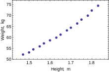
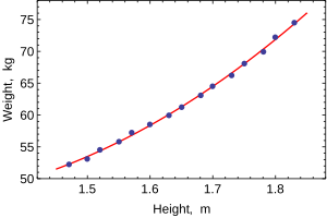
The following data set gives average heights and weights for American women aged 30–39 (source: The World Almanac and Book of Facts, 1975).

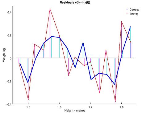
It might also reveal outliers, heteroscedasticity, and other aspects of the data that may complicate the interpretation of a fitted regression model.

These are some of the common diagnostic plots: An important consideration when carrying out statistical inference using regression models is how the data were sampled.

The fit of the model is very good, but this does not imply that the weight of an individual woman can be predicted with high accuracy based only on her height.