Propositional formula
The predicate calculus goes a step further than the propositional calculus to an "analysis of the inner structure of propositions"[4] It breaks a simple sentence down into two parts (i) its subject (the object (singular or plural) of discourse) and (ii) a predicate (a verb or possibly verb-clause that asserts a quality or attribute of the object(s)).
Synthesis: Engineers in particular synthesize propositional formulas (that eventually end up as circuits of symbols) from truth tables.
[6] Empiricists hold that, in general, to arrive at the truth-value of a synthetic proposition, meanings (pattern-matching templates) must first be applied to the words, and then these meaning-templates must be matched against whatever it is that is being asserted.
And maybe I am seeing a blue cow—unless I am lying my statement is a TRUTH relative to the object of my (perhaps flawed) perception.
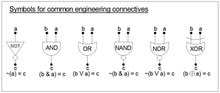
In their quest for robustness, engineers prefer to pull known objects from a small library—objects that have well-defined, predictable behaviors even in large combinations, (hence their name for the propositional calculus: "combinatorial logic").
[7] Thus an assignment of meaning of the variables and the two value-symbols { 0, 1 } comes from "outside" the formula that represents the behavior of the (usually) compound object.
The circuit mindlessly responds to whatever voltages it experiences without any awareness of TRUTH or FALSEHOOD, RIGHT or WRONG, SAFE or DANGEROUS.
For example, most people would reject the following compound proposition as a nonsensical non sequitur because the second sentence is not connected in meaning to the first.
On the other hand, logical equivalence sometimes appears in speech as in this example: " 'The sun is shining' means 'I'm biking' " Translated into a propositional formula the words become: "IF 'the sun is shining' THEN 'I'm biking', AND IF 'I'm biking' THEN 'the sun is shining'":[14] Different authors use different signs for logical equivalence: ↔ (e.g. Suppes, Goodstein, Hamilton), ≡ (e.g. Robbin), ⇔ (e.g. Bender and Williamson).
As noted above, Tarski considers IDENTITY to lie outside the propositional calculus, but he asserts that without the notion, "logic" is insufficient for mathematics and the deductive sciences.
For example, Hamilton uses two symbols = and ≠ when he defines the notion of a valuation v of any well-formed formulas (wffs) A and B in his "formal statement calculus" L. A valuation v is a function from the wffs of his system L to the range (output) { T, F }, given that each variable p1, p2, p3 in a wff is assigned an arbitrary truth value { T, F }.
They then verify their drawings with truth tables and simplify the expressions as shown below by use of Karnaugh maps or the theorems.
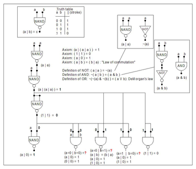
A complete analysis of all 2n combinations of truth-values for its n distinct variables will result in a column of 1's (T's) underneath this connective.
Thus the laws listed below are actually axiom schemas, that is, they stand in place of an infinite number of instances.
In general, to avoid confusion during analysis and evaluation of propositional formulas, one can make liberal use of parentheses.
Omitting parentheses with regards to a single-variable NOT: While ~(a) where a is a single variable is perfectly clear, ~a is adequate and is the usual way this literal would appear.
The inductive definition of infix formulas in the previous section can be converted to a formal grammar in Backus-Naur form: It can be shown that any expression matched by the grammar has a balanced number of left and right parentheses, and any nonempty initial segment of a formula has more left than right parentheses.
[19] It also locates the inner-most connective where one would begin evaluatation of the formula without the use of a truth table, e.g. at "level 6".
Some sophisticated tabular methods exist for more complex circuits with multiple outputs but these are beyond the scope of this article; for more see Quine–McCluskey algorithm.
This notion can be extended to three and four-dimensional hypercubes called Hasse diagrams where each corner's variables change only one at a time as one moves around the edges of the cube.
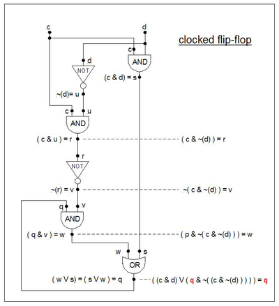
Example: ((c & d) ∨ (p & ~(c & (~d)))) = q in conjunctive normal form is: However, this formula be reduced both in the number of terms (from 4 to 3) and in the total count of its literals (12 to 6).
Use the values of the formula (e.g. "p") found by the truth-table method and place them in their into their respective (associated) Karnaugh squares (these are numbered per the Gray code convention).
In general there is no stipulation (either axiomatic or truth-table systems of objects and relations) that forbids this from happening.
To avoid this problem one has to know the state (condition) of the "hidden" variable p inside the box (i.e. the value of q fed back and assigned to p).
To understand [predict] the behavior of formulas with feedback requires the more sophisticated analysis of sequential circuits.
With the notion of "delay", this condition presents itself as a momentary inconsistency between the fed-back output variable q and p = qdelayed.
A truth table reveals the rows where inconsistencies occur between p = qdelayed at the input and q at the output.
A "row" instigated by William Hamilton over a priority dispute with Augustus De Morgan "inspired George Boole to write up his ideas on logic, and to publish them as MAL [Mathematical Analysis of Logic] in 1847" (Grattin-Guinness and Bornet 1997:xxviii).
About his contribution Grattin-Guinness and Bornet comment: Gottlob Frege's massive undertaking (1879) resulted in a formal calculus of propositions, but his symbolism is so daunting that it had little influence excepting on one person: Bertrand Russell.
Russell's work led to a collaboration with Whitehead that, in the year 1912, produced the first volume of Principia Mathematica (PM).