Radial basis function network
The output of the network is a linear combination of radial basis functions of the inputs and neuron parameters.
They were first formulated in a 1988 paper by Broomhead and Lowe, both researchers at the Royal Signals and Radar Establishment.
The norm is typically taken to be the Euclidean distance (although the Mahalanobis distance appears to perform better with pattern recognition[4][5][editorializing]) and the radial basis function is commonly taken to be Gaussian The Gaussian basis functions are local to the center vector in the sense that i.e. changing parameters of one neuron has only a small effect for input values that are far away from the center of that neuron.
Given certain mild conditions on the shape of the activation function, RBF networks are universal approximators on a compact subset of
[6] This means that an RBF network with enough hidden neurons can approximate any continuous function on a closed, bounded set with arbitrary precision.
There is theoretical justification for this architecture in the case of stochastic data flow.
Assume a stochastic kernel approximation for the joint probability density where the weights
It is sometimes convenient to expand the architecture to include local linear models.
is a Kronecker delta function defined as RBF networks are typically trained from pairs of input and target values
This step can be performed in several ways; centers can be randomly sampled from some set of examples, or they can be determined using k-means clustering.
A third optional backpropagation step can be performed to fine-tune all of the RBF net's parameters.
If the purpose is not to perform strict interpolation but instead more general function approximation or classification the optimization is somewhat more complex because there is no obvious choice for the centers.
The training is typically done in two phases first fixing the width and centers and then the weights.
Basis function centers can be randomly sampled among the input instances or obtained by Orthogonal Least Square Learning Algorithm or found by clustering the samples and choosing the cluster means as the centers.
The RBF widths are usually all fixed to same value which is proportional to the maximum distance between the chosen centers.
have been fixed, the weights that minimize the error at the output can be computed with a linear pseudoinverse solution: where the entries of G are the values of the radial basis functions evaluated at the points
The existence of this linear solution means that unlike multi-layer perceptron (MLP) networks, RBF networks have an explicit minimizer (when the centers are fixed).
In gradient descent training, the weights are adjusted at each time step by moving them in a direction opposite from the gradient of the objective function (thus allowing the minimum of the objective function to be found), where
For one basis function, projection operator training reduces to Newton's method.
The logistic map can be used to explore function approximation, time series prediction, and control theory.
The map originated from the field of population dynamics and became the prototype for chaotic time series.
The map, in the fully chaotic regime, is given by where t is a time index.
The examples here illustrate the inverse problem; identification of the underlying dynamics, or fundamental equation, of the logistic map from exemplars of the time series.
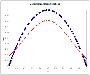
We choose the number of basis functions as N=5 and the size of the training set to be 100 exemplars generated by the chaotic time series.
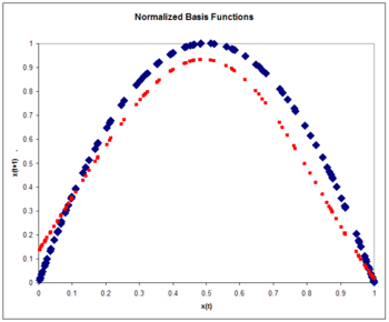
The normalized RBF architecture is where Again: Again, we choose the number of basis functions as five and the size of the training set to be 100 exemplars generated by the chaotic time series.
This is a property of the sensitive dependence on initial conditions common to chaotic time series.
A measure of the divergence of time series with nearly identical initial conditions is known as the Lyapunov exponent.
We assume the output of the logistic map can be manipulated through a control parameter
such that The goal is to choose the control parameter in such a way as to drive the time series to a desired output
This can be done if we choose the control parameter to be where is an approximation to the underlying natural dynamics of the system.