Space-filling curve
In mathematical analysis, a space-filling curve is a curve whose range reaches every point in a higher dimensional region, typically the unit square (or more generally an n-dimensional unit hypercube).
[1][2][3][4][5][6] Intuitively, a curve in two or three (or higher) dimensions can be thought of as the path of a continuously moving point.
To eliminate the inherent vagueness of this notion, Jordan in 1887 introduced the following rigorous definition, which has since been adopted as the precise description of the notion of a curve: In the most general form, the range of such a function may lie in an arbitrary topological space, but in the most commonly studied cases, the range will lie in a Euclidean space such as the 2-dimensional plane (a planar curve) or the 3-dimensional space (space curve).
It is also possible to define curves without endpoints to be a continuous function on the real line (or on the open unit interval (0, 1)).
Peano was motivated by Georg Cantor's earlier counterintuitive result that the infinite number of points in a unit interval is the same cardinality as the infinite number of points in any finite-dimensional manifold, such as the unit square.
The problem Peano solved was whether such a mapping could be continuous; i.e., a curve that fills a space.
Therefore, Peano's space-filling curve was found to be highly counterintuitive.
From Peano's example, it was easy to deduce continuous curves whose ranges contained the n-dimensional hypercube (for any positive integer n).
It was also easy to extend Peano's example to continuous curves without endpoints, which filled the entire n-dimensional Euclidean space (where n is 2, 3, or any other positive integer).
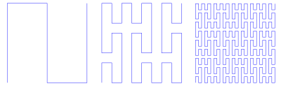
Most well-known space-filling curves are constructed iteratively as the limit of a sequence of piecewise linear continuous curves, each one more closely approximating the space-filling limit.
Peano's ground-breaking article contained no illustrations of his construction, which is defined in terms of ternary expansions and a mirroring operator.
But the graphical construction was perfectly clear to him—he made an ornamental tiling showing a picture of the curve in his home in Turin.
His choice to avoid any appeal to graphical visualization was motivated by a desire for a completely rigorous proof owing nothing to pictures.
At that time (the beginning of the foundation of general topology), graphical arguments were still included in proofs, yet were becoming a hindrance to understanding often counterintuitive results.
A year later, David Hilbert published in the same journal a variation of Peano's construction.
[8] Hilbert's article was the first to include a picture helping to visualize the construction technique, essentially the same as illustrated here.
The analytic form of the Hilbert curve, however, is more complicated than Peano's.
is a continuous function mapping the Cantor set onto the entire unit square.
(Alternatively, we could use the theorem that every compact metric space is a continuous image of the Cantor set to get the function
in the construction of the Cantor set, we define the extension part of
to be the line segment within the unit square joining the values
[9] For the classic Peano and Hilbert space-filling curves, where two subcurves intersect (in the technical sense), there is self-contact without self-crossing.
A space-filling curve's approximations can be self-avoiding, as the figures above illustrate.
In 3 dimensions, self-avoiding approximation curves can even contain knots.
Roughly speaking, differentiability puts a bound on how fast the curve can turn.
Michał Morayne proved that the continuum hypothesis is equivalent to the existence of a Peano curve such that at each point of the real line at least one of its components is differentiable.
There are many natural examples of space-filling, or rather sphere-filling, curves in the theory of doubly degenerate Kleinian groups.
For example, Cannon & Thurston (2007) showed that the circle at infinity of the universal cover of a fiber of a mapping torus of a pseudo-Anosov map is a sphere-filling curve.