Wave function

In one common form, it says that the squared modulus of a wave function that depends upon position is the probability density of measuring a particle as being at a given place.

The integral of a wavefunction's squared modulus over all the system's degrees of freedom must be equal to 1, a condition called normalization.

, now called the De Broglie relation, holds for massive particles, the chief clue being Lorentz invariance,[14] and this can be viewed as the starting point for the modern development of quantum mechanics.

Those who used the techniques of calculus included Louis de Broglie, Erwin Schrödinger, and others, developing "wave mechanics".

Those who applied the methods of linear algebra included Werner Heisenberg, Max Born, and others, developing "matrix mechanics".

[18] This was shown to be incompatible with the elastic scattering of a wave packet (representing a particle) off a target; it spreads out in all directions.

In 1927, Hartree and Fock made the first step in an attempt to solve the N-body wave function, and developed the self-consistency cycle: an iterative algorithm to approximate the solution.

There are several advantages to understanding wave functions as representing elements of an abstract vector space: The time parameter is often suppressed, and will be in the following.

Then utilizing the known expression for suitably normalized eigenstates of momentum in the position representation solutions of the free Schrödinger equation

[nb 5] Following are the general forms of the wave function for systems in higher dimensions and more particles, as well as including other degrees of freedom than position coordinates or momentum components.

All the previous remarks on inner products, momentum space wave functions, Fourier transforms, and so on extend to higher dimensions.

In the case of non separable Hamiltonians, energy eigenstates are said to be some linear combination of such states, which need not be factorizable; examples include a particle in a magnetic field, and spin–orbit coupling.

Generally, bosonic and fermionic symmetry requirements are the manifestation of particle statistics and are present in other quantum state formalisms.

For N distinguishable particles (no two being identical, i.e. no two having the same set of quantum numbers), there is no requirement for the wave function to be either symmetric or antisymmetric.

Substituting the form of wavefunction in Schrodinger's time dependent wave equation, and taking the classical limit,

The Dirac (or interaction) picture is intermediate, time dependence is places in both operators and states which evolve according to equations of motion.

where R are radial functions and Ymℓ(θ, φ) are spherical harmonics of degree ℓ and order m. This is the only atom for which the Schrödinger equation has been solved exactly.

The wave functions represent the abstract state characterized by the triple of quantum numbers (n, ℓ, m), in the lower right of each image.

This motivates the introduction of an inner product on the vector space of abstract quantum states, compatible with the mathematical observations above when passing to a representation.

In summary, the set of all possible normalizable wave functions for a system with a particular choice of basis, together with the null vector, constitute a Hilbert space.

More generally, one may consider a unified treatment of all second order polynomial solutions to the Sturm–Liouville equations in the setting of Hilbert space.

All of these actually appear in physical problems, the latter ones in the harmonic oscillator, and what is otherwise a bewildering maze of properties of special functions becomes an organized body of facts.

In this case, as well, the part of the wave functions corresponding to the inner symmetries reside in some Cn or subspaces of tensor products of such spaces.

Not all introductory textbooks take the long route and introduce the full Hilbert space machinery, but the focus is on the non-relativistic Schrödinger equation in position representation for certain standard potentials.

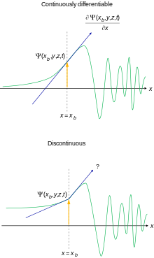
The following constraints on the wave function are sometimes explicitly formulated for the calculations and physical interpretation to make sense:[45][46] It is possible to relax these conditions somewhat for special purposes.

[47] Note that exceptions can arise to the continuity of derivatives rule at points of infinite discontinuity of potential field.

The normalization condition requires ρ dmω to be dimensionless, by dimensional analysis Ψ must have the same units as (ω1ω2...ωm)−1/2.

Many famous physicists of a previous generation puzzled over this problem, such as Erwin Schrödinger, Albert Einstein and Niels Bohr.

Some advocate formulations or variants of the Copenhagen interpretation (e.g. Bohr, Eugene Wigner and John von Neumann) while others, such as John Archibald Wheeler or Edwin Thompson Jaynes, take the more classical approach[49] and regard the wave function as representing information in the mind of the observer, i.e. a measure of our knowledge of reality.

Some, including Schrödinger, David Bohm and Hugh Everett III and others, argued that the wave function must have an objective, physical existence.